Balancing the weight of variables in a decision tree

Sometimes, when facing the challenge of modelling the operation of a process where different variables are involved, we find that some of them dominate over the others. These variables will thus exert greater influence compared to the rest. Let us take, for example, processes with declarative data where the variable to be predicted is informed by the actual user. A typical case for a continuous variable might be a home value estimator that can take any numerical value and request information on a form from the user as ranges of values. For instance, with  a drop-down field containing different options. In this case, the information declared can be expected to almost entirely describe the variable to be predicted. The purpose of using an estimator on an already known data can be very varied: to make a discrete variable continuous, to smooth a variable, to detect data entry errors, to refine the declared data to unify criteria, or simply to comply with a regulation.

The importance of a variable can be calculated in different ways depending on the type of model being fitted. For example, in a Linear or Logistic Regression it is usually related to the weight (coefficient) associated with each descriptor variable, while in the case of trees it is usually related to the reduction of the metric used to make the splits. There are also model agnostic techniques; one of the best known is Permutation Feature Importance¹. This technique is usually used in models that are already trained, poorly interpretable or highly non-linear. Furthermore, it is based on randomly breaking the relationship between the descriptor variable and the target variable, observing the consequent decrease in the model performance. In any case, regardless of how the importance of a variable in a model is measured, the measurement result in some way represents the dependence between the model output and the variable in question.

In an industrialised process where the output of a model is used to make decisions, it is generally bad practice to over-rely on a low number of variables as these might fail to be reported (or may be misreported) due to technical failure. In such cases, the prediction will be more or less reliable based on the dependence of these same variables. The home value estimator, for example, is highly dependent on the data provided. Therefore, the variable will be misreported if, for instance, the form’s format or data type is updated. This would effectively cause the estimator to generate wholly erroneous outputs.

Another important point is that a model that is highly dependent on one variable can easily be violated, thus causing a potential problem in the acceptance process. Going back to our previous example, let us now assume that the estimated home value provides access to credit, and that the estimator is highly dependent on the average income declared by the user. In other words, the higher the average income, the higher the value of the home. In case this relationship is detected, the estimator can easily be tricked by simply inflating the average income value. This will, in turn, lead to erroneous access to credit.

For the above reasons, diluting the importance of variables in a model makes it robust against failures and attacks. On the other hand, the model generally suffers in terms of performance.

In the case of Linear Regression, it is sometimes possible to impose hard constraints on the coefficients in the optimisation process ², as well as penalties on the magnitude of the coefficients. However, in the case of decision trees, there is no similar procedure available that applies to the model building algorithm.

A common alternative is to introduce random noise on the dominant variable, trying to strike a balance between decreasing predictive power and the variable’s contribution to the model. It would also be possible to randomly limit the subset of candidate variables in each division of the tree. This, however, presents the disadvantage of leaving the selection ordering and the resulting error metric reduction to chance. Another alternative would be to order this selection by using an error metric that does not select variables that over-contribute during the initial steps of the decision, thereby limiting their importance. However,  this is not a simple procedure as it implies knowing from the outset the extent to which each variable reduces the error.

This last solution, however, sounds reasonable due to the fact that the most important variables come into play during the latter stages of the decision process. This solves the problems outlined at the beginning and means that resulting model would not be so dependent on this type of variable.

In our use case we only had one highly significant variable (~90% in error reduction). The rest of the variables were more or less balanced in terms of importance. We therefore decided to approximate the above solution with a simple procedure we refer to as Extended Trees. This consists of two steps: first, fit a regression tree with all variables except the one with the highest importance, and then extend the leaves of the previous tree using only the variable left out in the previous step.

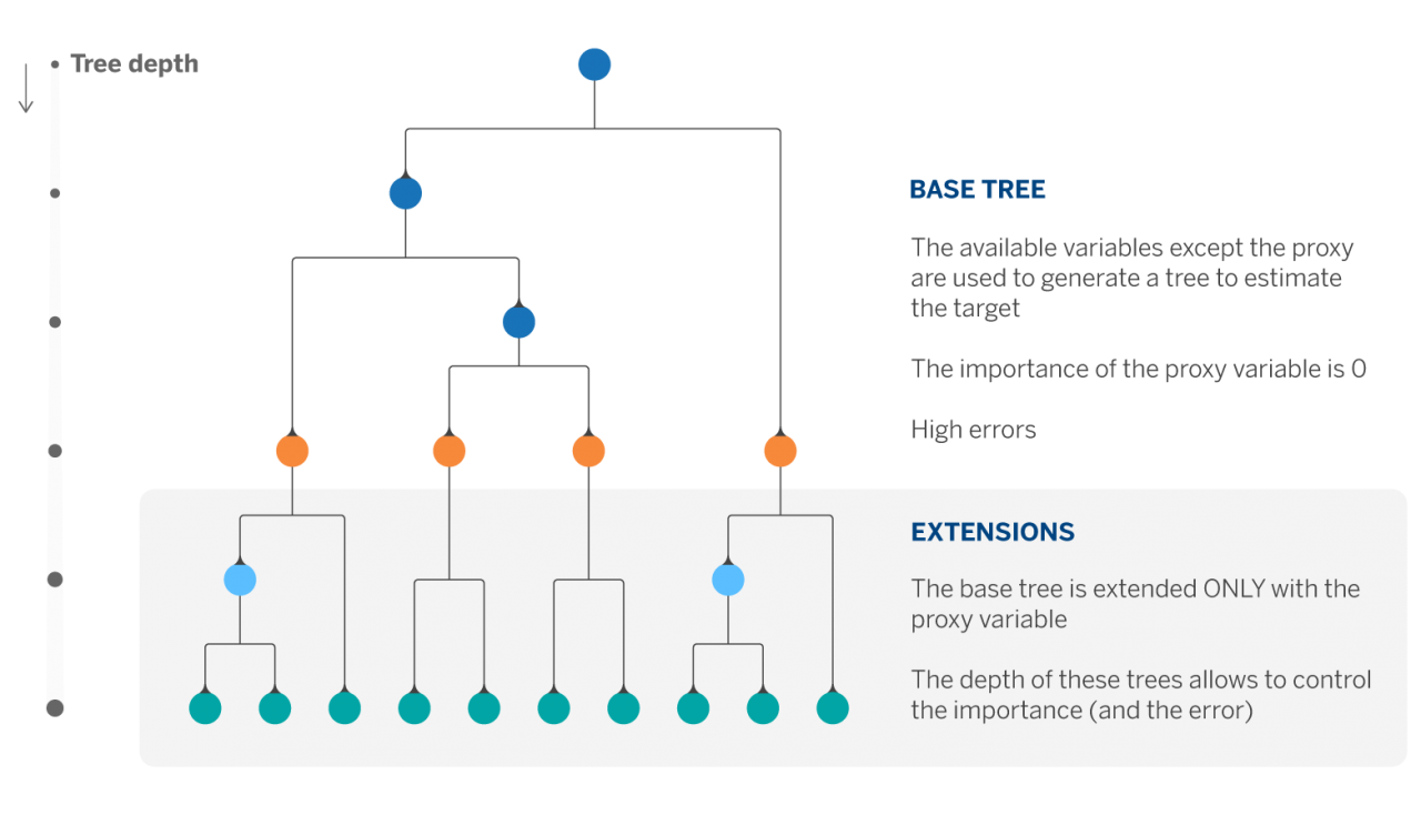
The hyper-parameter set consisting of the depth of the first tree and the depths of the n extents (where n is the number of leaves of the first tree) allows us to control the contribution of the variable whose importance we wish to limit.

By using this approach in our problem we manage to reduce the importance of the proxy variable by ~45% and increase the original error by 3%.

California Housing dataset

In order to better understand this procedure, we show an example application on the California Housing database. It was constructed from the housing census and each entry corresponds to a block group, the smallest geographical unit for which the US census publishes information (typically composed of 600 to 3,000 inhabitants). In total, the dataset consists of 20,640 observations, 8 numerical variables and the target variable, which are: median income (MedInc), median age of dwellings (HouseAge), median number of rooms (AveRooms) and bedrooms (AveBedrms), population, average occupancy of dwellings (AveOccup), latitude and longitude. As well as the variable we are going to predict, which is the median value of the dwellings in a block group.

The following figure shows the importance of each descriptor variable after training a Decision Tree Regressor (DTR) of depth 4 (in blue) and an ExtendedTree (ExT) of initial depth 3 and extension depth 2 (in orange), in order to estimate the median value of the dwellings of each block group. In both cases, the cross-validation technique has been used to obtain the results.

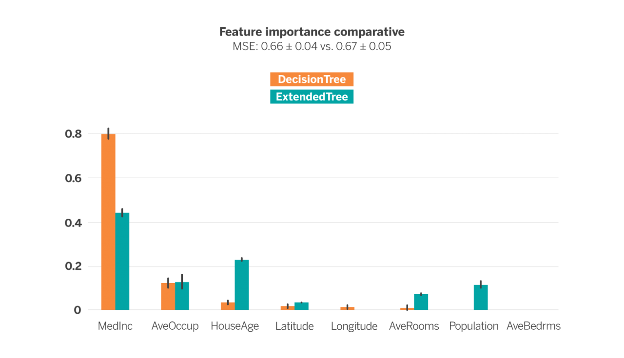
The error metric used is the Mean Squared Error (MSE), whose use is very common in the evaluation of the performance of regression models. In this case, both models have been configured so that the error metric is as similar as possible (0.66 ± 0.04 vs. 0.67 ± 0.05), i.e. trying to ensure that both estimators perform equally well in estimating the median value of the dwellings from the available variables. Such a configuration results in a 31-node tree in the case of DTR and the 61-node tree in the case of ExT. As we can see, the latter is much more complex than the former at equal error.

If we look at the importance of each variable in each model (represented by the height of the bar) we see that the DTR is ~80% dependent on the MedInc variable, the next most important variable is AvgOccup with just under 20% and the rest of the variables barely influence the estimation of the model. In the case of ExT, however, the most important variable is still MedInc but at just over 40%, with the importance being more evenly distributed among the other variables.

It is worth highlighting the case of the HouseAge, AveRooms and Population variables. While in the DTR they have hardly any influence, in the ExT their importance is not negligible. This means that they are valuable variables for price estimation. However, in the case of the DTR they are overshadowed by MedInc. In short, the ExT is able to exploit more uniformly the available variables, while maintaining the error in exchange for generating a more complex structure.

In conclusion, depending on the nature of the data, ExtendedTrees can be a simple solution to the problem of high dependency in Decision Tree models. This mechanism can also be applied in the case of classification. Moreover, ExtendedTrees are easy to understand. Their output structure is the same as that of a Decision Tree, and they allow for the contribution of each variable in a tree to be controlled, within the possibilities and by means of depths. Nevertheless, they can bring about an increase in error or complexity.