Designing strategies to cope with classification problems: a Quick Study

Building artificial intelligence models involves several stages, including training and evaluation. To ensure that the models perform correctly, data scientists must select metrics to evaluate the models after training. This is a complex task: some metrics are more appropriate than others, depending on the use case.

Evaluation metrics have advantages and disadvantages that must be evaluated before implementation, so there is no consensus on whether one metric is better than another for evaluating models. In this sense, metrics are usually chosen ad hoc for each use case. Since the problems are addressed individually, they require an exhaustive work of computation with different metrics and, consequently, a significant investment of time and effort.

At BBVA AI Factory, we wanted to establish a common strategy that would allow us to have a guide for using metrics so that each time we evaluate a model, we can identify which is the most appropriate. This proposal arises in the context of classification problems, specifically on multiclass and multilabel classification models. To implement it, we conducted a quick study, one of the initiatives of exploration and innovation with data that we have established in the AI Factory.

Motivation of the Quick Study: Multiclass and Multilabel Problems

A quick study, as its name suggests, is a theoretical study on a specific problem carried out in a short time. These studies try to reach valid conclusions for several teams, so they have a certain degree of transversality and lead to knowledge sharing to define common strategies. These strategies consider state-of-the-art innovative techniques that can be extrapolated to different use cases.

The first Quick Study conducted at the BBVA AI Factory aims to address the problem of evaluating multiclass and multi-label models. Several teams in our hub work on classification problems, so the need to compare different evaluation techniques and lay the groundwork for a cross-cutting proposal became apparent.

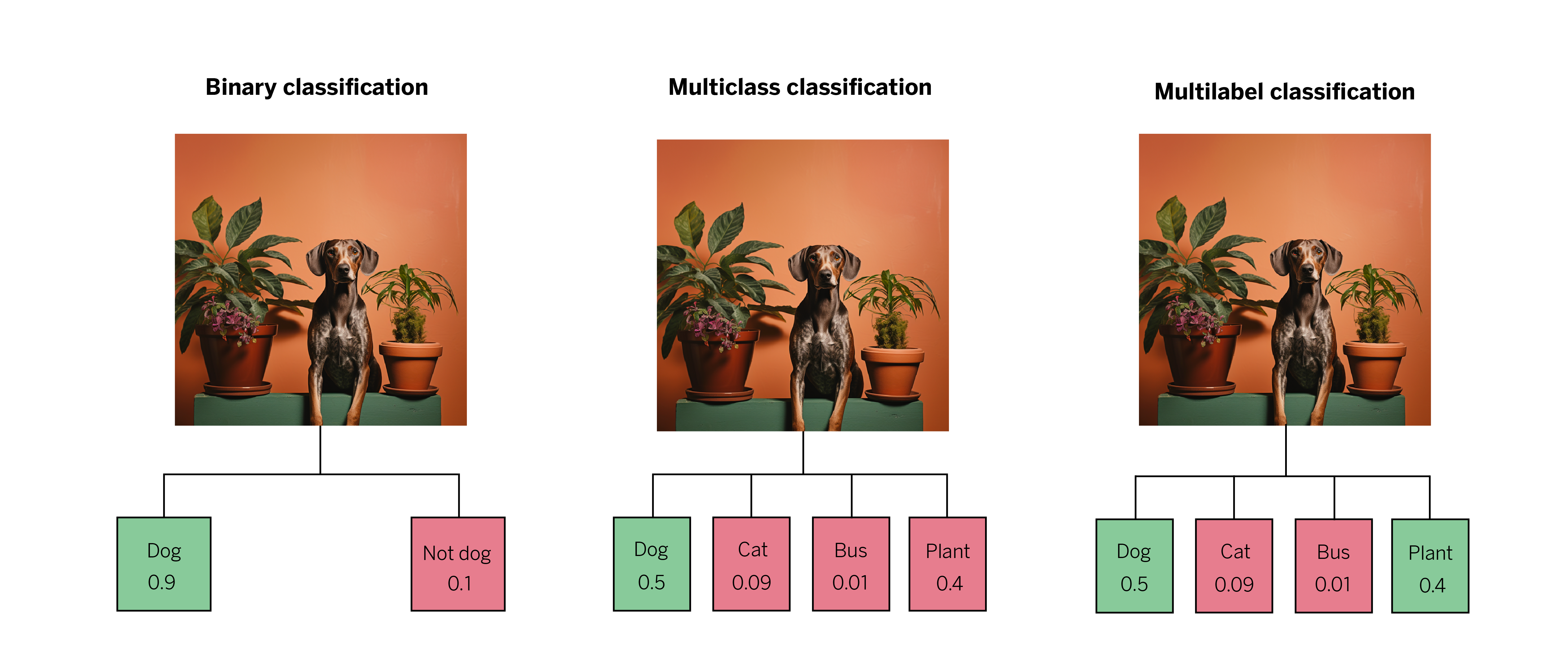
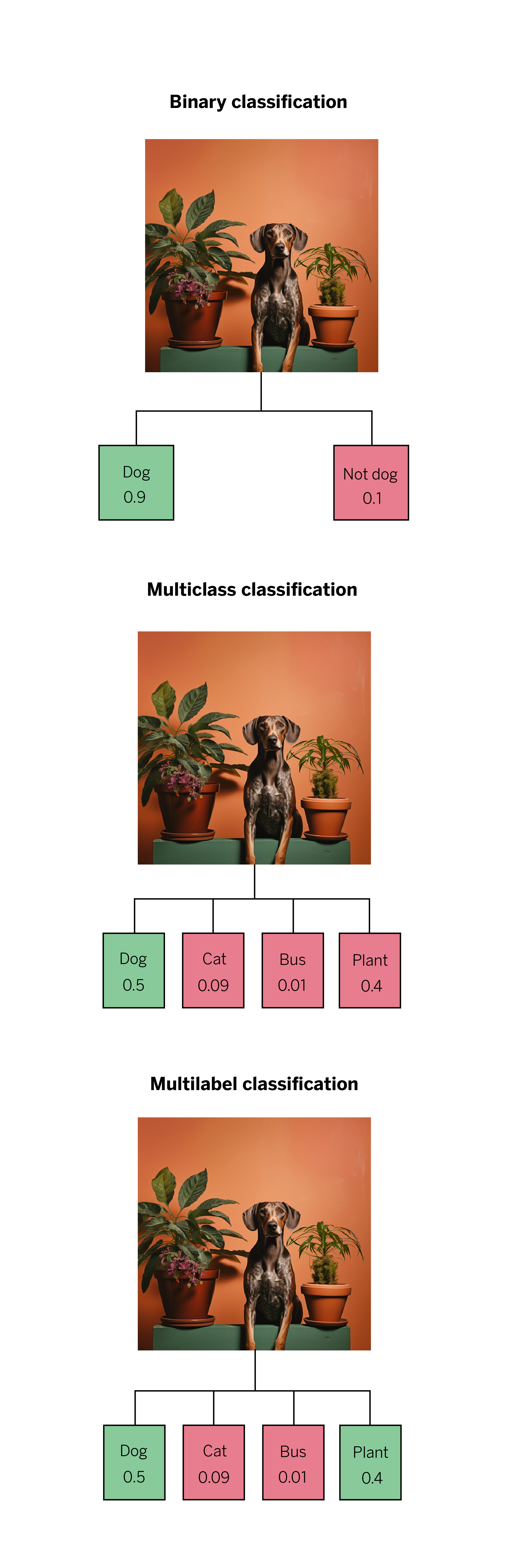
Multiclass problems are those where we have multiple labels available for each sample. Still, in the end, only a single label is associated with each observation or sample on which a single prediction is made. An example to illustrate this: we see a picture of a dog next to a plant, and we have the labels “dog,” “cat,” “bus,” and “plant.” The model will identify only one of the items as true, even though both are in the image. This type of model only associates the label it has learned as the most likely: in this case, the dog.

On the other hand, multi-label problems allow more than one label for each sample. In this case, returning to the previous example, the model can partially succeed, such as identifying the dog and the plant. This means that it can assign some, all, or none of the labels, depending on the quality of the model and the classification problem it faces.

One of the use cases that motivated this quick study is the classification problem that arises in conversations between customers and BBVA managers through the bank’s application. When determining which product is being discussed, there is a multi-label problem since the same conversation can be assigned different products and, therefore, different labels.

We have a taxonomy – or set of topics – of 14 possible products associated with the conversations. To train our model, we have a sample of labeled conversations, but there is a problem: the distribution of products is not equal, since, for example, the volume of conversations about “accounts” and “cards” (products within the taxonomy) is not equal to the volume of conversations about “payroll” or “warranties” (less common).

Several modeling strategies have been tried to solve this problem:

1. Using the labeled sample without balancing worsened the results for the minority products.
2. Trying to balance the volume of all products leads to worse results for the majority products.
3. Trying to balance the quantity of majority and minority products. This strategy did not produce the best results for either the majority or minority products.

Faced with choosing one modeling strategy or another, we focused on metrics. Each of the above strategies presents a set of metrics (at an individual product level and an overall model level) that get better or worse depending on what we are looking at. Finally, we ask ourselves: Which of the tested metrics should we stick with?

Understanding the Advantages and Disadvantages of Each Metric in Multiclass Problems¹

In the context of classification problems (both binary, multiclass, and multi-label), we need to distinguish between hard and soft predictions. Soft prediction refers to the estimated probability that an observation belongs to one of the classes. In contrast, hard prediction refers directly to the class predicted by the model for a sample. Also, we have to consider that multiclass problems involve several labels, of which only one is assigned to an observation. All in all, we have two typologies of metrics, depending on what we want to evaluate.

• Quality of hard predictions
• Quality of soft predictions

We assume there is no bad metric, but its advantages and disadvantages depend on the goal we want to achieve in a use case.

Quality of Hard Predictions

We will go into each of the metrics that help us determine the quality of hard predictions to know their function, formula, advantages, and disadvantages.

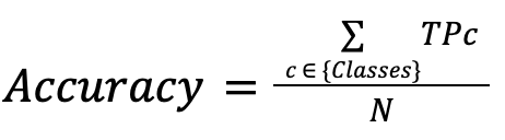
Accuracy

It indicates how many correctly classified observations are out of the total observations.

Advantages	Disadvantages
It is useful when we aim to classify as many samples as possible.	The classes that are more represented in our dataset will have more weight in the metric, so it will not be helpful, for example, to guarantee a good performance in minority classes.

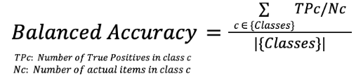
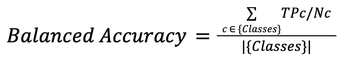
Balanced Accuracy

Measures each class’s accuracy individually, then averages them by dividing by the number of classes.

Advantages	Disadvantages
This is useful when you want the model to perform equally well in all classes since all classes have the same weight, so it helps improve performance in the less-represented classes.	If the classes have different importance, this metric may not be very convenient if we are interested in having a good prediction in the dataset as a whole.

Balanced Accuracy Weighted

Measures the accuracy of each class and then averages them using specific weights.

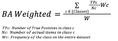
Advantages	Disadvantages
Each class is assigned a specific weight so that it can be adapted to the needs of each use case.	In real-world problems, determining the weight of each class is often difficult and may not reflect reality well.

Micro Average (precision, recall, f1)

All observations are considered together, so hits are measured overall, regardless of class.

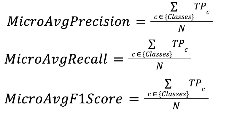
Advantages	Disadvantages
Same as Accuracy.	Same as Accuracy.

Macro Average (precision, recall, f1)

The average of the metrics (precision, recall, f1) in each individual class is considered.

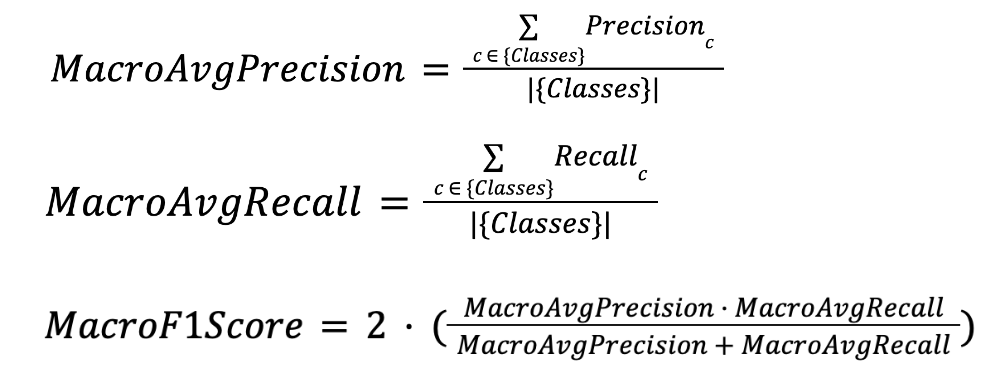
Advantages	Disadvantages
Same as Balanced Accuracy.	Same as Balanced Accuracy.

Weighted Average (precision, recall, f1)

Parts of the Macro Average formulas by multiplying each Precision or Recall by the user-defined weight of each class.

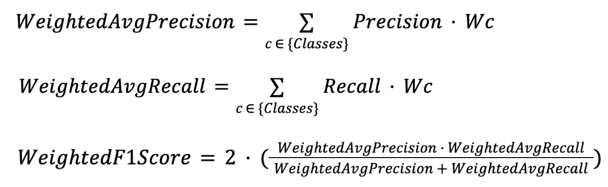
Advantages	Disadvantages
Same as Balanced Accuracy Weighted.	Same as Balanced Accuracy Weighted.

Mattheus Correlation Coefficient

Formula based on the relationship between correctly and incorrectly classified items.

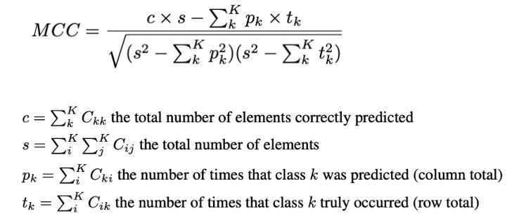
Advantages	Disadvantages
More robust to class imbalance problems.	Not very interpretable. Although the contribution of the most represented classes is attenuated, they still carry more weight.

Cohen’s Kappa

Measures the closeness of the predicted classes to the actual classes by comparing the model to a random classification according to the distribution of each class.

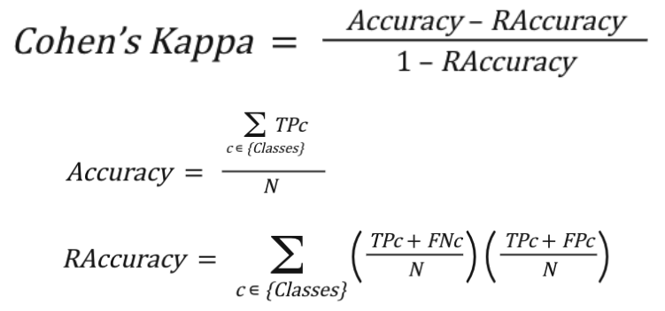
Advantages	Disadvantages
Can correct for biases in overall accuracy when dealing with unbalanced data.	Poorly interpretable. The further away the training distribution is from the actual distribution, the less we can compare these metrics, so different unbalancing strategies cannot be tested.

Accuracy

It indicates how many correctly classified observations are out of the total observations.

Advantages
It is useful when we aim to classify as many samples as possible.

Disadvantages
The classes that are more represented in our dataset will have more weight in the metric, so it will not be helpful, for example, to guarantee a good performance in minority classes.

---

Balanced Accuracy

Measures each class’s accuracy individually, then averages them by dividing by the number of classes.

Advantages
This is useful when you want the model to perform equally well in all classes since all classes have the same weight, so it helps improve performance in the less-represented classes.

Disadvantages
If the classes have different importance, this metric may not be very convenient if we are interested in having a good prediction in the dataset as a whole.

---

Balanced Accuracy Weighted

Measures the accuracy of each class and then averages them using specific weights.

Advantages
Each class is assigned a specific weight so that it can be adapted to the needs of each use case.

Disadvantages
In real-world problems, determining the weight of each class is often difficult and may not reflect reality well.

---

Micro Average (precision, recall, f1)

All observations are considered together, so hits are measured overall, regardless of class.

Advantages
Same as Accuracy.

Disadvantages
Same as Accuracy.

---

Macro Average (precision, recall, f1)

The average of the metrics (precision, recall, f1) in each individual class is considered.

Advantages
Same as Balanced Accuracy.

Disadvantages
Same as Balanced Accuracy.

---

Weighted Average (precision, recall, f1)

Parts of the Macro Average formulas by multiplying each Precision or Recall by the user-defined weight of each class.

Advantages
Same as Balanced Accuracy Weighted.

Disadvantages
Same as Balanced Accuracy Weighted.

---

Mattheus Correlation Coefficient

Formula based on the relationship between correctly and incorrectly classified items.

Advantages
More robust to class imbalance problems.

Disadvantages
Not very interpretable. Although the contribution of the most represented classes is attenuated, they still carry more weight.

---

Cohen’s Kappa

Measures the closeness of the predicted classes to the actual classes by comparing the model to a random classification according to the distribution of each class.

Advantages
Can correct for biases in overall accuracy when dealing with unbalanced data.

Disadvantages
Poorly interpretable. The further away the training distribution is from the actual distribution, the less we can compare these metrics, so different unbalancing strategies cannot be tested.

Quality of Soft Predictions

Next, we will look at each of the metrics that help us determine the quality of soft predictions to understand their functions, advantages, and disadvantages.

Cross-entropy

Measures the distance between the results and the original distributions.

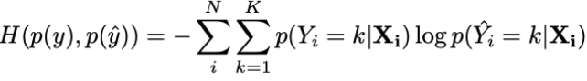
Advantages	Disadvantages
It is an appropriate method when we are interested in having an excellent overall performance of our scores.	It does not evaluate the quality of the classification rule.

ROC Curves

Constructs ROC curves for each class and then calculates the area under these curves to average or weight them.

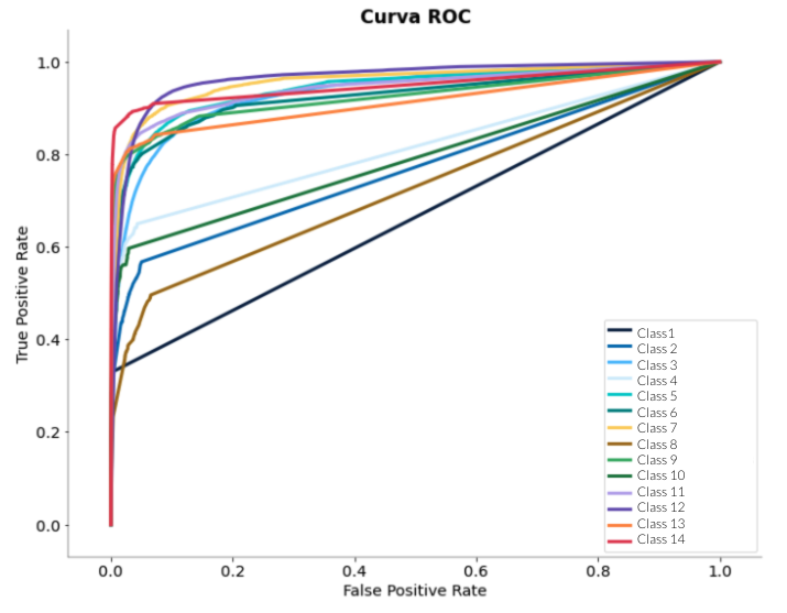
Advantages	Disadvantages
By visualizing the curves, we can decide the cutoff we want to use for classification.	It requires a probability model. Its robustness to changes in the distribution of classes can be a disadvantage if the data set is unbalanced.

Precision-recall curves

The area under these curves is calculated and averaged or weighted.

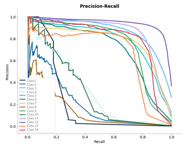
Advantages	Disadvantages
By visualizing the curves, we can decide the cutoff we want to use for classification.	Requires a probability model.

Cross-entropy

Measures the distance between the results and the original distributions.

Advantages
It is an appropriate method when we are interested in having an excellent overall performance of our scores.

Desventajas
It does not evaluate the quality of the classification rule.

---

ROC Curves

Constructs ROC curves for each class and then calculates the area under these curves to average or weight them.

Advantages
By visualizing the curves, we can decide the cutoff we want to use for classification.

Desventajas
It requires a probability model. Its robustness to changes in the distribution of classes can be a disadvantage if the data set is unbalanced.

---

Precision-recall curves

The area under these curves is calculated and averaged or weighted.

Advantages
By visualizing the curves, we can decide the cutoff we want to use for classification.

Disadvantages
Requires a probability model.

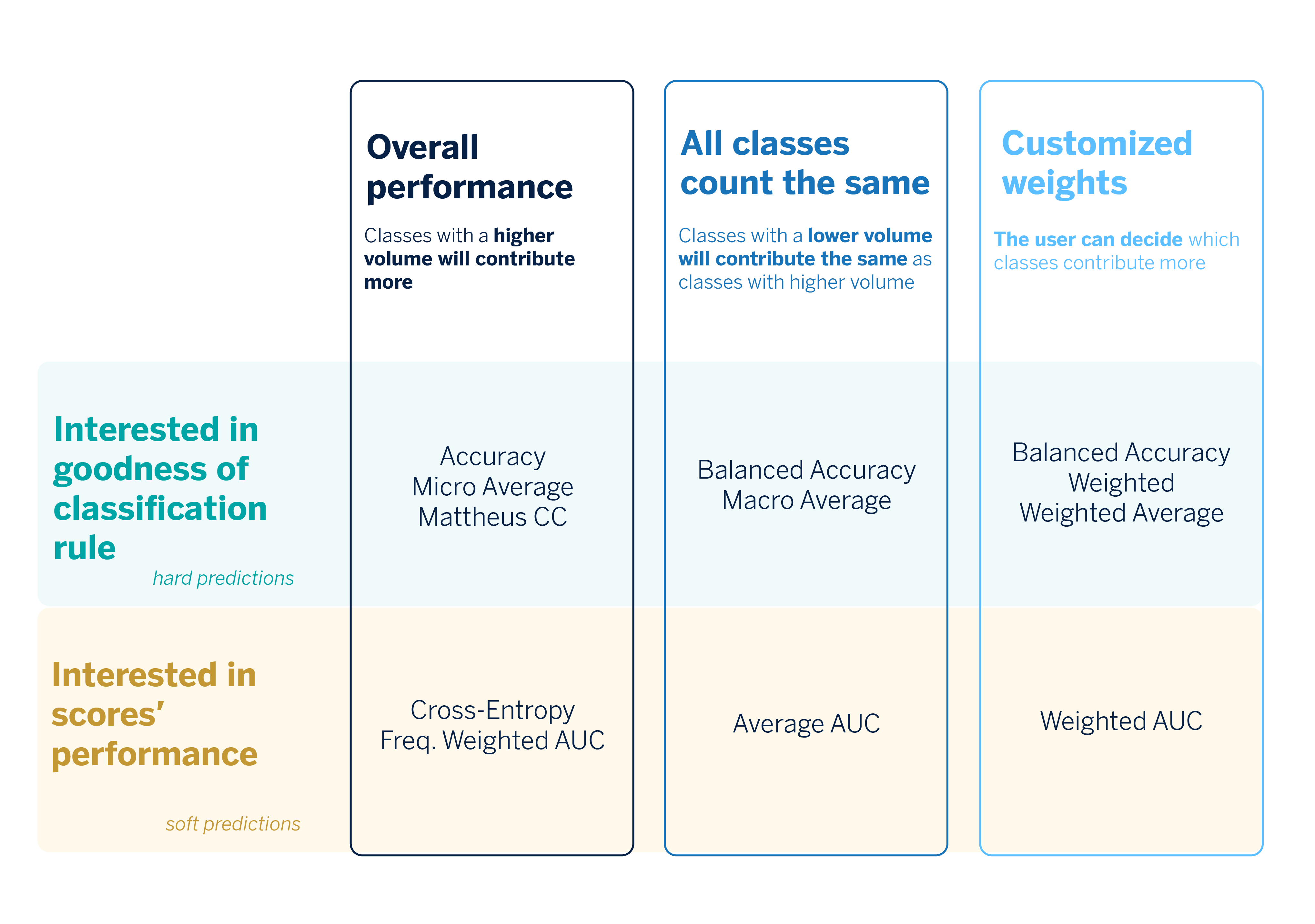
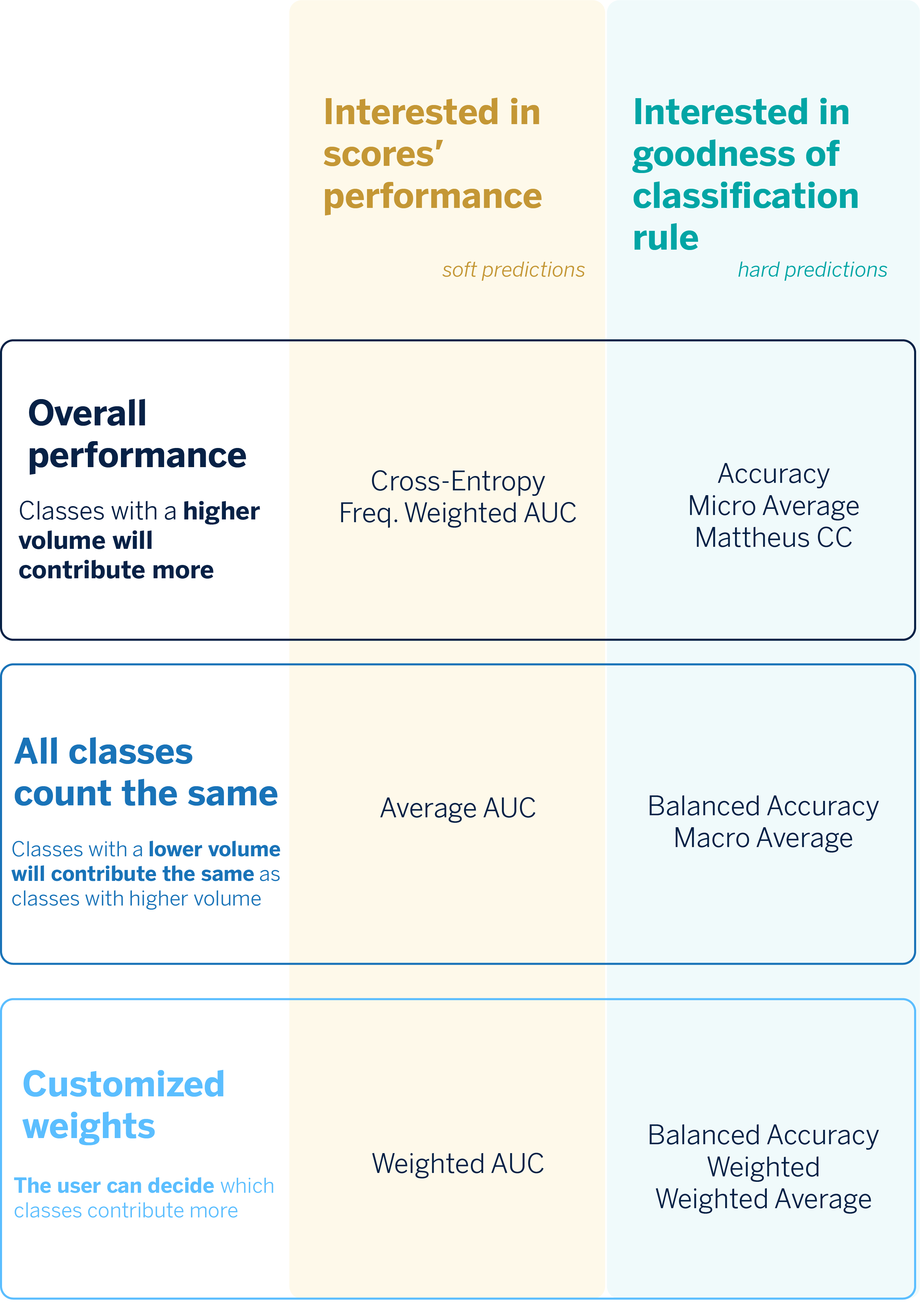
Once we have a broader idea of what each metric does, we can provide a summary guide of the metrics we should use to tackle multiclass classification problems.

Multi-label problems: Possible Strategies

In multi-label problems, classes are not exclusive; they can coexist. An observation can have more than one label associated with it. Thus, the strategy of using metrics is different. However, a cross-cutting problem involves both multilabel and multiclass models: classes may be unbalanced. In the multi-label case, this can be even more pronounced because the more labels that are assigned to each observation, the more the prediction can be affected if they are unbalanced.

To try to address these issues and to explain the types of metrics that can help us evaluate multilabel models, we have found three types of strategies in the literature:^2,3

Ranking-based

This strategy can help us if, in addition to assigning a label to an observation, we want to rank the labels according to their relevance or probability. This metric type can be helpful when the model output is a list of ordered labels.

This strategy is particularly useful in extreme classification scenarios and when we want to use more straightforward metrics (e.g. ranking loss, one-error, propensity versions). It is also helpful for building recommendation systems. However, many use cases do not fit the fact that the model output is in ranking format.

Label-based

It consists of considering the multilabel problem as a set of multiclass problems. This strategy aims to compute the performance in each class and then compute some aggregation through averages or weighted averages.

It allows us to evaluate and average the predictive performance of each class as a binary classification problem. Still, it does not consider the distribution of labels per observation. Also, classes are not random samples, so the result is only sometimes consistent when we average the classes.

Example-based

This is a set of metrics calculated by averaging over observations rather than classes. Some of these metrics are based on set theory (e.g., Jaccard Score or Hamming Loss).

It consists of calculating, for each sample, the closeness between the predicted and true label sets. While it solves the specificity problem concerning samples or observations, it does not consider the specificity of unbalanced classes in extreme classification problems.

Computing metrics: Exercise with scikit-multilearn

To complement our research, we performed a practical exercise consisting of the following:

1. We use the scikit-learn datasets module to generate synthetic data corresponding to a multilabel classification problem. This module is parameterized so that the number of observations and labels can be varied.
2. Using the scikit-multilearn library,⁴ and following the Binary Relevance approach, we easily and quickly train models with different degrees of complexity (e.g., from a Support Vector Classifier to a Gaussian Process Classifier).
3. For each candidate model, we compute the metrics for multilabel problems described above (ranking-based, label-based, and sample-based) and summarize them in tabular form for easier comparison. We also compute the training time (fit_time) and the prediction time (pred_time) for informational purposes in the case latency is also significant in our use case.

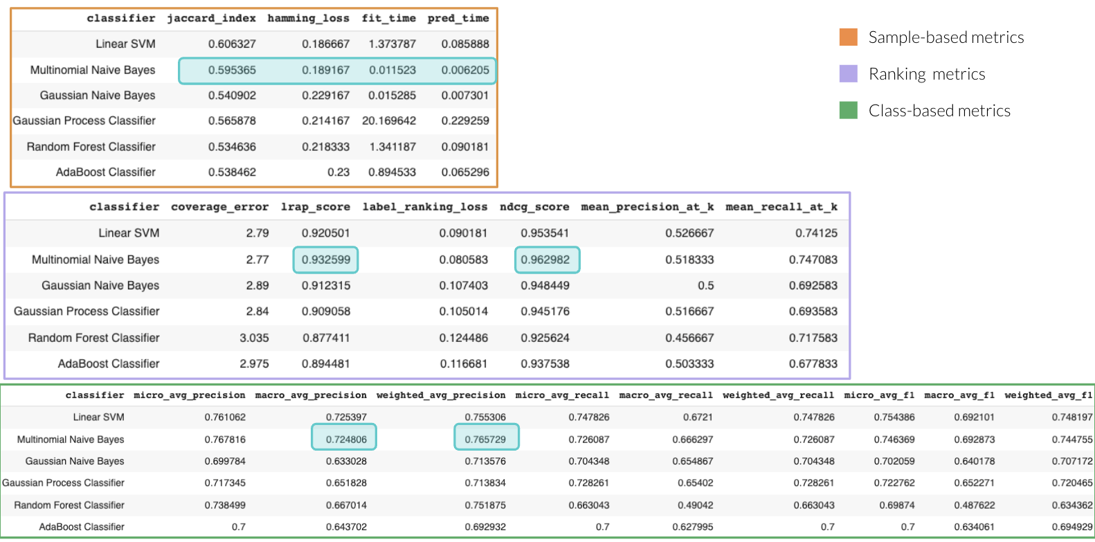
Once we have all the metrics computed, we can create two-dimensional graphs by selecting the metrics we are interested in comparing and thus observe how each model performs, look explicitly at the tradeoffs, and be able to choose the one that best suits our needs.

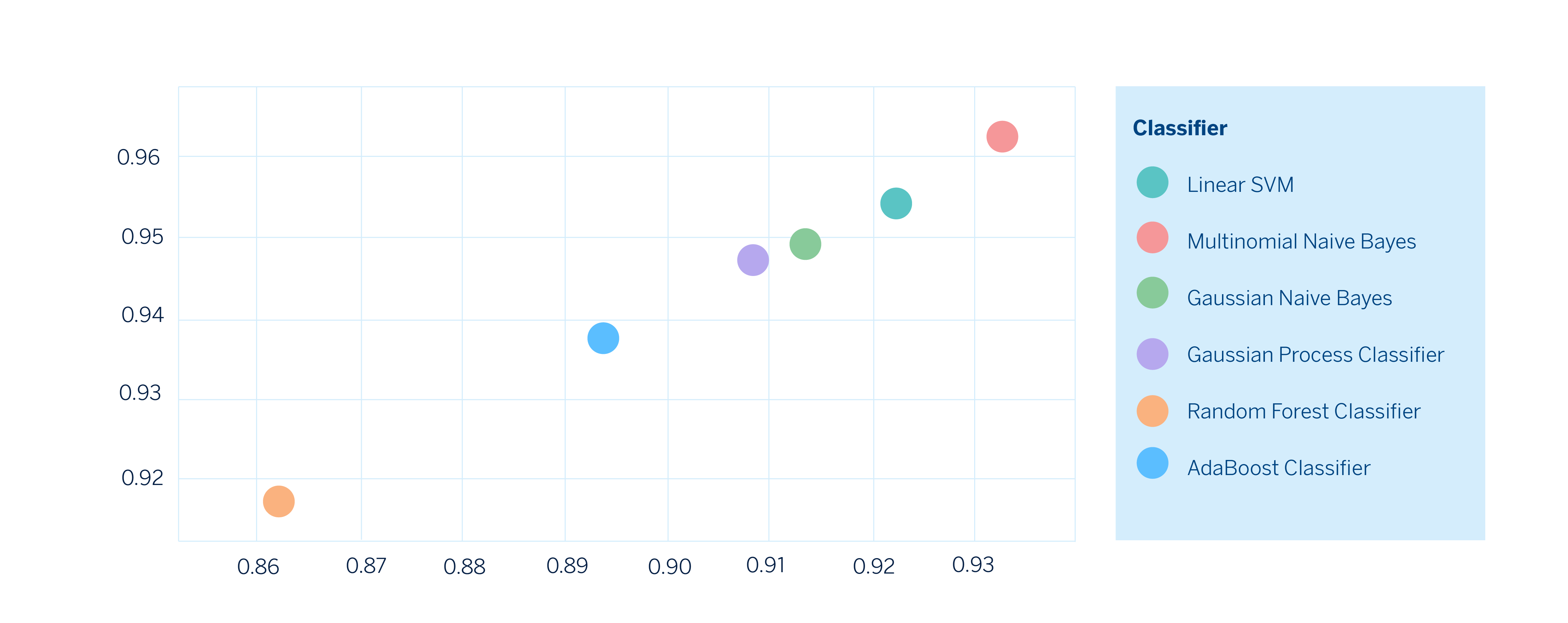
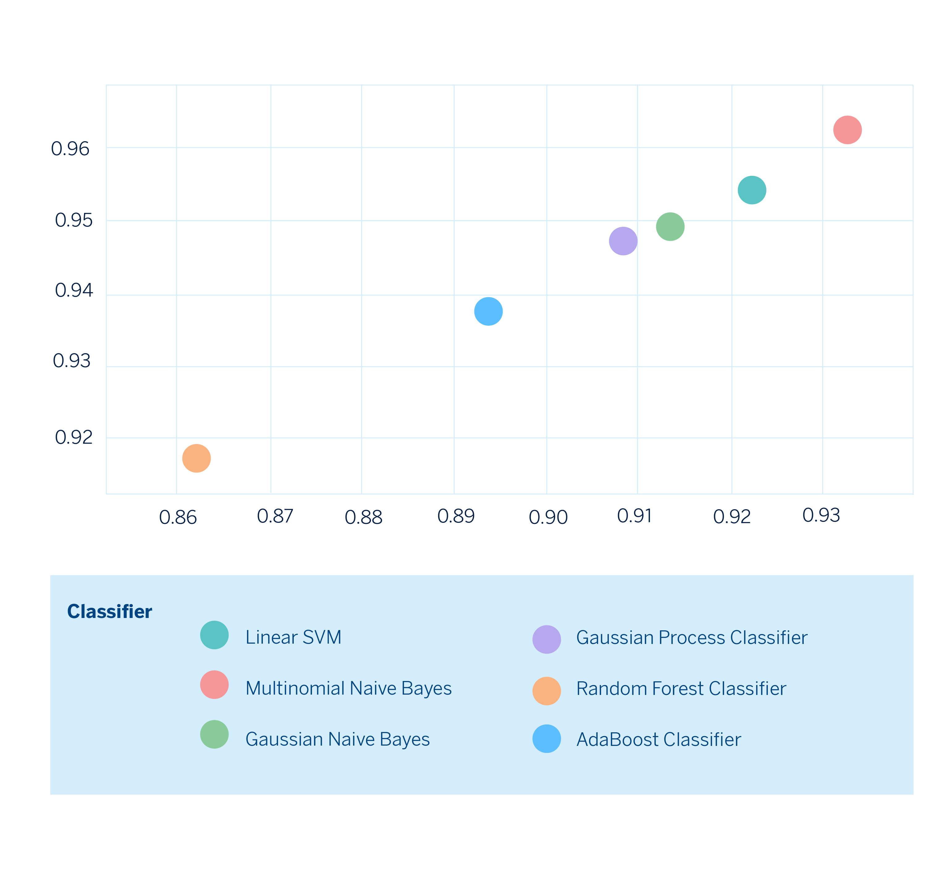
Finally, we can select the model that best fits our needs. In this hypothetical scenario, the model built with Multinomial Naive Bayes would perform best on both metrics.

Conclusions

The main conclusion is clear: there are no good or bad metrics, it all depends. It depends on the use case, and it depends on the relevance of the weight of a variable, it depends on the number of labels associated with an observation. However, we have created a roadmap for dealing with multiclass cases and are extending our techniques for multi-label problems.

All this work on finding techniques that can be applied to different use cases shows us that reality is much more complex, so there are problems that cannot be solved with the same strategies. However, gathering information that helps us build a comprehensive protocol for dealing with classification problems is a step forward in our journey to create more personalized experiences.