No existe algo llamado “predicción segura”

One question that naturally springs up when imagining what Artificial Intelligence (AI) can bring to the banking industry, and one that we get asked fairly often, is: Can you predict people’s expenses? As it is often the case, such a simple question is in fact only apparently simple. The prediction of personal financial transactions may range from estimating the amount of your next electricity bill (a simple problem, in most cases), all the way to guessing the time and amount of your next ATM withdrawal (a seemingly impossible task, in most cases).

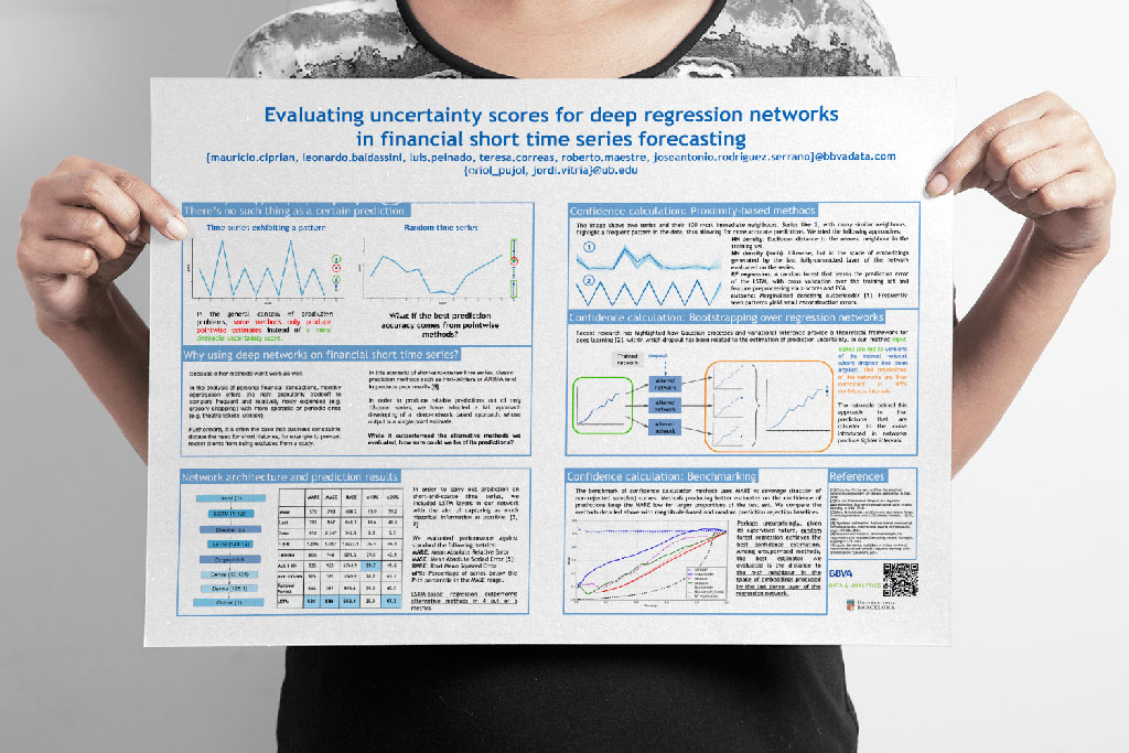
With all its inherent difficulties, anticipating the behaviour of personal accounts is a challenge that holds a special place in any modern platform of intelligent banking services. For this reason, we have been investigating the best way to tackle this problem. This week we are presenting some results in the Workshop on Machine Learning for Spatiotemporal Forecasting as part of the NIPS 2016 conference. Our contribution is entitled Evaluating uncertainty scores for deep regression networks in financial short time series forecasting¹ . Here is a walk-trough:

Keep it short

To use a jargon common to both statistics and Machine Learning, we were facing a time-series regression problem, something that, normally, any trained statistician would not even blink at. However, a detail made our problem setting perceivably harder than usual: Its coarseness. In the analysis of personal financial transactions, it often makes sense to aggregate data at a monthly timescale, since many important financial events only happen with a monthly cadence (think payroll), or a multiple thereof (think utility bills), or would introduce excessive noise in the data if considered at a finer level (think grocery shopping). Furthermore, we wanted to be able to predict expenses for as many clients as possible, including those having relatively short financial histories. This forced us to work on just a year-worth of data with monthly aggregations. In other words, for each client and transaction category, we only had 12 historical values. We had to guess the 13th.

While this class of problems has been widely studied, especially for long series, some of the best-suited statistical methods for these prediction problems, such as Holt-Winters or ARIMA, tend to produce poor results on such short time series. This led us to look at our problem from a different perspective, that of Machine Learning.

If it flies like a duck…

Instead of trying to predict the 13th value in our series solely by looking at each of them individually, as classical time series methods would normally do, we adopted a common underlying principle in many Machine Learning algorithms:

If it looks like a duck, swims like a duck and quacks like a duck, then it probably is a duck.

This disarmingly informal statement (sometimes referred to as the duck test) is a humorous phrasing of a common methodology of machine learners: If a target time series is sufficiently similar to training time series whose 13th value is known, then the behaviour observed in the training series should help us guess how the target series will evolve.

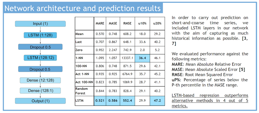
We therefore started experimenting with classic approaches directly leveraging this principle, such as Nearest Neighbour regression and Random Forest regression. Worryingly, under most of our error metrics these supposedly cleverer methods were severely losing to much naiver solutions such as predicting by taking an arithmetic mean of the series, or simply by using the value 0 for all predictions (an effect of the sparsity of many financial time series). It was clear that in those short 12-values sequences, there was more structure than these methods were able to capture.

In order to squeeze as much information as possible from our short series, in a collaboration with the University of Barcelona we developed a deep neural network which employed Long Short-Term Memory (LSTM) units in order to exploit their power to remember past information, a property that makes them useful tools to learn sequential structures.

The margin of improvement was evident.The next figure compares error and success metrics of different prediction methods, including our LSTM network.

An odd duck

While greatly improved, the error-metrics values were still high. Higher than you’d want for any client-facing application ready to be released into the world.

An often underestimated implication of the duck-test approach is that if a target series doesn’t really have any other series that looks akin, many algorithms will still stubbornly output a prediction – only, it will be unreliable. It goes without saying that an uncertainty score (or confidence value) accompanying a prediction is a highly desirable feature for an algorithm, but one that deep networks, including ours, usually lack (a matter of very active research).

In order to estimate the uncertainty of our deep-network predictions, we turned our attention to a few quantities we could compute that were reminiscent of the concept of uncertainty. For example, while computing the distance to the nearest time series was not the most accurate prediction method, the distance to the most closely-looking series can be considered a proxy of prediction uncertainty (duck test!), as can the reconstruction error of a marginalised denoising autoencoder or the distance between the representation of a series that can be found in the last layer of our LSTM network (an idea that proved greatly successful in the field of Computer Vision). To further add to our list of uncertainty-estimation methods, we also tried a supervised approach by training a Random Forest to learn prediction errors directly.

Finally, we applied the duck-test principle to prediction models, rather than to the data: If a target series gets similar predictions from models that have been partially corrupted by noise, this means that the original model is sufficiently confident of its knowledge of the series’s pattern. We implemented this approach by applying dropout noise on the trained network, hence bootstrapping 95% confidence intervals on our predictions.

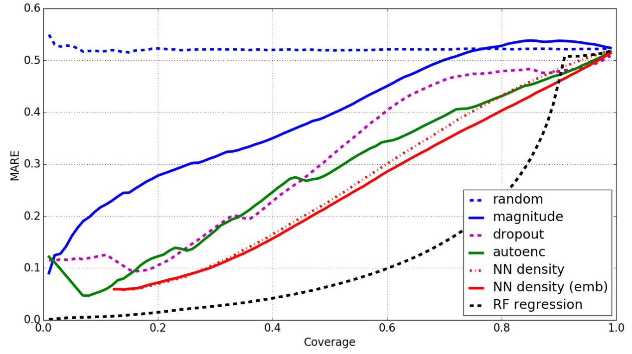
For the benchmark of confidence calculation methods we used Mean Absolute Relative Error vs coverage (fraction of non-rejected samples) curves. Intuitively, this means that methods producing better prediction-uncertainty estimates keep the MARE low for larger proportions of the test set. Note that this allows us to filter out the series which the algorithm is not confident about, leaving us with a much cleaner dataset to use in production environments.

We compared the different confidence calculation methods we implemented with simple rejection baselines, such as estimating uncertainty only by looking at the absolute value of predictions or by a completely random value. Perhaps unsurprisingly, given its supervised nature, random forest regression achieved the best confidence estimation. Among unsupervised methods, the best estimator we evaluated is the distance to the n-th neighbour in the space of embeddings produced by the last dense layer of the regression network. We found it interesting that the density in the network embedding space is a relatively good proxy of the uncertainty.