Financial Text Classification: Methods for Word Embedding

Text classification is at the center of many business challenges we tackle at BBVA Data & Analytics. Categorization of an account transaction is one of the most rewarding and applicable solutions and has gradually grown into one of the most powerful assets of BBVA’s award-winning mobile app. Assigning an operation to an expense category is fundamental for personal finance management applications, allowing, for instance, to browse expenses by meaningful categories such as ”household”, ”insurances” or ”travel”. Moreover, it adds a semantic layer from which other applications can benefit (e.g. forecasting by expense category). This is a technical summary of the teachings and insights obtained working with word embeddings for the categorization of short sentences for financial transactions.

In machine learning, the text classification problem is defined as follows: given a dataset of pairs (s_j , c_j ) where s_j is a string of text and c_j is one of the possible labels or categories for the given text, we aim at learning the function or classifier F mapping an arbitrary string of text to one of the possible labels.

Introduction to Word Embeddings

In order to solve any of the text classification problems mentioned, a natural question arises: How do we treat text computationally? In order to do this, data scientists treat the text as a mathematical object. Over the years, machine learning researchers have found ways to transform words into points of a Euclidean space of a certain dimension. This transformation is called “embedding”, which assigns a unique vector to each word appearing in our vocabulary.

With this mathematical transformation, we enable new operations on words that were previously not possible: in a given space (of D dimensions) we can add, subtract, and dot multiple vectors, among many other operations.

Therefore, in order to evaluate an embedding, it is desirable for these ”new” operations to be capable of translating the words into semantic properties that were not obvious prior to the embedding. In particular, in most embeddings, the scalar product of normalized vectors (cosine similarity) is used as a similarity function between words.

Implicitly, most non-trivial word embeddings rely on the distributional hypothesis, which states that words that occur in the same context have similar meanings. While this holds mostly true (it can produce really meaningful embeddings when given enough text, as we will see), it appears to be something that you can draw conclusions on only when you have seen enough text. In fact, we will explore some flaws of the methods that assume this hypothesis when not enough text is available. This is the same idea of what happens sometimes in statistics when the sample is not large enough. The distribution of the sum of the results of rolling a fair dice twice will not resemble a normal distribution as much as the distribution of rolling 100 will do.

Another interesting problem that cannot be covered in this post is how to combine word vectors to form vector representations of sentences. Although this was part of my research in 2018, in this post I use the simple approach of normalizing the average of word vectors. While not always the best performing method, this approach is the most natural mathematical construction.

Count vs predict embedding and “privileged information”²

There are numerous ways to learn the embedding of a word. A possible distinction of the different embedding techniques is between context-count based embeddings and context-prediction based embeddings. This depends on whether the vectors are obtained by counting word appearances or by predicting words within given contexts. The former – more traditional models – rely mostly on factorizing matrices obtained by counting appearances of words and the contexts they appear in, while the latter try to predict a word based on its context (or vice-versa), mostly using neural methods. Note that both these types of embeddings try to extract information from a word using its context, and therefore implicitly rely on the distributional hypothesis. A good explanation for the matrix factorization count-based methods can be found here.

Additionally, given the fact that our final goal is text classification, there is also another possible difference between embedding methods. Since the dataset used to embed the words is labeled, one could theoretically use the sentence labels to create more meaningful embeddings. The community sometimes refers to these methods as having access to “privileged information”, an idea which is also used in computer vision to rank images.

Some examples of Word Embeddings

Bag of Words

The most trivial Word Embedding is known as Bag of Words (BoW). It consists of mapping each word from a vocabulary V = {w_j}_j∈N  as a one-hot encoded vector; in other words, a vector containing all zeros, except a 1 at the position corresponding to the index representing the word.

There are several drawbacks that immediately follow from the definition, yet this simple embedding is fairly efficient in terms of performance, as we will show later.

Some downsides of BoW are the inability to choose the embedding dimension, which is fixed by the size of the vocabulary, and the sparsity and dimension of the resulting embedding since the vocabulary size can be potentially very large. However, the most important differentiating factor between this Bag Of Words embedding and others is that this model only learns from the vocabulary, and not from any text of the dataset. This means that it is unable to learn any notion of similarity other than distinguishing whether or not two words are different (with this encoding, all words are equidistant).

Metric Learning

A possible improvement to the BoW is an embedding that tunes the BoW vectors by learning a metric that is able to differentiate sentences in our dataset by their labels. Hence, we will refer to this as Metric Learning. Looking at the labels means Metric Learning is having access to supervised information with a deeper understanding of the similarities among similar words.

In a nutshell, metric learning starts from a data-free embedding (such as BoW) and proposes a transformed embedding. Such a transformation is performed in a way in which the embeddings of sentences of the same class appear close to one another, and far from the embeddings of other classes in the transformed space. This gives rise to a word embedding that takes into account the semantic information provided by sentence labels.

Word2Vec

On the other hand, the most widely used unsupervised embedding is Word2Vec,  presented by ex-Googler Tomas Mikolov. It learns word embeddings by trying to predict a word given its context (Continuous Bag of Words) or by trying to predict a context given the word (Skip-Gram), being, therefore, context-predicting and relying on the distributional hypothesis. It has achieved very good performance in several text-related tasks, since, given enough text, cosine similarity highly accurately detects synonyms in texts and perhaps more surprisingly embeddings carry enough information to solve problems such as “Man is to Woman as Brother is to ?” with vector arithmetic, since the vector representation of “Brother” – ”Man” + ”Woman” produces a result which is closest to the vector representation of “Sister”. This fact was also cleverly used to reduce biases in embeddings. It is the perfect example of how embeddings can take advantage of the structure of the Euclidean space to obtain more information about the words impossible to detect in the original word space.

Word Embeddings in practice

In this section I will introduce some results concerning the usage of Word Embeddings learned during the internship:

• Heuristics to a certain when word2vec has learned an acceptable solution.
• On small datasets, one can use metric learning with small amounts of supervised sentences and obtain word embeddings of the same quality as those of Word2vec trained with up to millions of sentences.

While we consider these anecdotal, we were not aware of these insights in the literature, this is why we are sharing them here.

Word2Vec training insights

These insights mostly deal with choosing the correct amount of epochs while training a Word2vec model, and thus to define a metric and hypothesize concerning the behavior of Word2vec’s learned synonyms when insufficient data is available.

The number of epochs that a word2vec model has to be trained is a hyperparameter which can sometimes be difficult to tune. However, using the evolution of the similarity matrix MtM, where M is the normalized embedding matrix can give us a sense of whether our word2vec has already learned good vector representations or not. Recall that  (M_tM)ij = similarity(wi, wj ) and −1 < (M_tM)ij < 1 and so it is not desirable that most of the values of the matrix values are high. Ideally, we would only want synonym pairs to have high similarity. Experimentally, as it can be shown in Figure 1, the squared sum of non-diagonal elements of MtM squared is shown to first increase and later decrease until stabilizing. Note that this is not in any way be a replacement for the loss function, nor a lower value means a better-trained model: the BoW model satisfies ||M^tM – Id||^2_F = 0, but it obviously fails to capture word similarities.

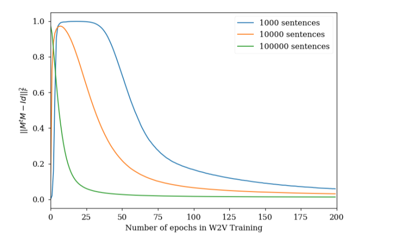
This behavior can be interpreted as follows: first of all, the model randomly initializes the vectors assigned to each word, It then moves most of these to the same region of the embedding space. Subsequently, as the model sees different words in different contexts, it starts separating them until only the synonyms are close together (because they were moved the same way). To confirm this hypothesis, some more analyses should be carried out related to how the angle distribution of vectors changes with training. However, training Word2vec with a small number of words and looking at the synonyms found can provide evidence of similar behavior to the one described.

As already mentioned, Word2vec provides highly accurate synonyms or two different representations of the same word, such as “third” and “3rd” using cosine similarity of normalized vectors. This is because when the model has seen enough text, it learns to identify that the contexts of “third” and “3rd” are very similar most of the time and, therefore, does not separate the vectors. However, when insufficient data is provided (or the model is not trained for enough epochs), the found synonyms (those pairs of vectors with a cosine similarity) sometimes show a behavior not found in fully trained embeddings: Words that the model has always seen together are treated as synonyms. For example, if a small amount of text often contains “BBVA Data”, but then does not contain any examples of “BBVA” without “Data” or vice versa, the model will likely not distinguish between these two words because they always appear in the same context. Therefore, the model will assign to them high similarity (because it relies on the distributional hypothesis). This can be useful for determining that more text or more training is needed. In conclusion, thinking of word2vec as separating all vectors and keeping only close words instead of only joining similar words can be useful in determining whether or not our embedding is fully trained.

In the following gif animation, we show the evolution of the matrix M^tM with training. This is shown to help develop an intuition of the training process. In the animation, lower indices correspond to more frequent words, and it is observed how the model is able to differentiate between them with fewer epochs.

Supervised vs Unsupervised Word Embeddings in small datasets

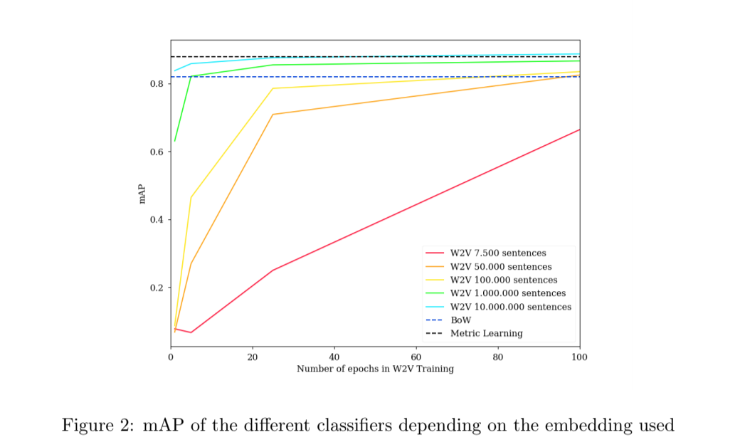
Additionally, an experiment was performed to evaluate Word Embeddings in the specific conditions of a small dataset of short questions. In a dataset of around 20,000 Stack Overflow categorized questions, labeled as one of 20 different categories. BoW and Metric Learning embeddings were trained using the sentences in the dataset and used to label the sentences by training a logistic regression classifier. Additionally, using a large amount of Stack Overflow unlabelled questions, different Word2Vecs are trained, each time using a different amount of sentences, including sentences from the dataset itself. Mean average precision is used as the metric to compare between the classifiers. The results can be found in Figure 2. As can be seen, a very large amount of sentences are needed for word2vec to outperform Metric Learning. Even training a word2vec with 2.5 times the amount of sentences from the original dataset does not significantly outperform BoW. In conclusion, BoW and especially Metric Learning, are far more suitable in cases when not a great deal text from a particular kind is available. It is commonly agreed in the literature that predict-based word embeddings are superior to any other embeddings. However, in this particular case of a small dataset of short sentences, a more classical approach yielded better results.

Conclusions and acknowledgments

For some applications, a large amount of text can be difficult to acquire, and therefore, there is a case to be made for Metric Learning or other similar embeddings which performed well while using only the small amount of data from the dataset itself.

My summer internship at BBVA Data & Analytics was a fantastic learning experience and helped me dive deep into the basics of Natural Language Processing, with the guidance of great professional mentors. Most of all, I would like to thank José Antonio Rodríguez for its time and patience supervising both of my internships in the company and for all the new concepts that he has taught me.