How to tag data faster using Active Learning

With Artificial Intelligence we are able to translate texts automatically, search for a similar image on Google, or even draw; however, until these systems are able to learn things by themselves, they will continue to depend on humans for preparing, cleaning and labelling the data that feeds them. When we turn to an AI system to automate a task, such as translating a text, it is because a team of humans have fed it with thousands or millions of verified inputs (sentences in the original language) and outputs (sentences in the desired language), a process known as tagging. This mode of Artificial Intelligence is known as supervised learning.

At BBVA AI Factory we design data products based on Machine Learning models with the aim of automating tasks that provide value to users, such as classifying bank transactions or detecting the degree of urgency of a customer message. For these tasks, we face the challenge of having to prepare and label datasets.

Whether the labels can be obtained in some intelligent way, or -in the worst case- they have to be entered manually, obtaining a labeled dataset of sufficient quality or size is one of the bottlenecks of Machine Learning systems. This is done to the point that we sometimes help with data labelling without even being aware of it¹.

For this reason, we recently launched a project to prototype a fast annotation system. The ingredient to achieve this is a statistical technique called “active learning”.

	This prototype is the first to be developed within the X Program, an internal exploration and innovation initiative awarded by Fast Company, which extends its recognition to BBVA AI Factory as one of the 100 Best Workplaces for Innovators, and the winner in the category of “Small Companies” (2022). Read more →

This prototype is the first to be developed within the “X Program”, an internal exploration and innovation initiative awarded by Fast Company, which extends its recognition to BBVA AI Factory as one of the 100 Best Workplaces for Innovators, and the winner in the category of “Small Companies” (2022). Read more →

Prototyping active learning

Active learning is an automatic technique that allows the person tagging data to know which items have the most valuable tags. This is a technique that dates back almost to the beginnings of Machine Learning and has been shown in studies to be able to reduce the amount of data to be annotated. However, until recently, most of the literature was limited to academic studies with few existing documented examples of state-of-practice² or industrial systems.

Why Active Learning works

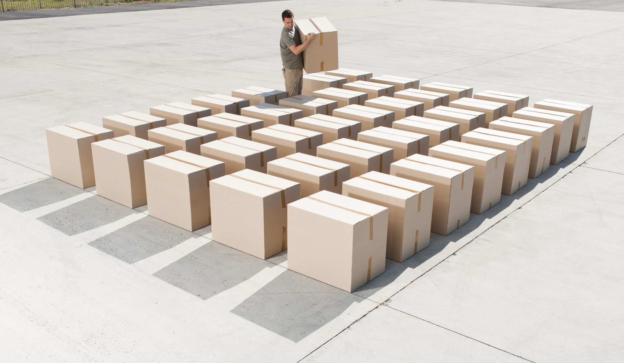
Let’s explain better why active learning works with a simple example. Let us imagine that we have several closed boxes on the floor inside a room. From the outside, these boxes are exactly the same, but on the inside they are painted in a certain color. Our mission is to ascertain what color paint is on the inside of the boxes and to annotate this information. In short, we have a set of data (the boxes) and we want to write down their characteristics or information (color). The simplest and most direct way to do this is to open one box at a time and see what color the inside is painted in.

In the example above we can easily open all the boxes and annotate their labels, because there are only two attributes (their position on the x and y axes) and a limited set of boxes. But the fact of the matter is that in our day-to-day life we face more complex datasets and hence we need a way to achieve a satisfactory performance without having to invest too much effort in labelling. Returning to the example of the boxes, when we have a lot of boxes to open, the process can take us longer than expected and we may have to call on several friends to help us with the task. The question then arises: would it be possible to know the color of most of the boxes quicker without having to open them all?

In our case, we know that the order in which the boxes are placed is not random, but that their position is related to the color inside. We intuit, therefore, that we should eventually be able to distinguish different zones of boxes according to their color, although we cannot determine this before we start opening them. Thus, using supervised learning and the information of the position of the boxes, we are going to try to discover their colors more efficiently. The goal of supervised learning is to anticipate the point of separation between the blue box area and the red box area. Although we have very few boxes labeled according to their color, we ask a Machine Learning classifier model (random forest) to try to separate the two regions. The model makes a first separation between this areas, predicting which boxes would be of which color. To improve the reliability and predictions of the model, we have to open some more boxes.

The advantage of using active learning is that the model itself suggests which box (data to be labeled) we should open next. In other words, instead of randomly choosing the next piece of data to be labeled, by using active learning we know what data can provide us with more information to improve the model prediction. In this way, the new boxes to be opened and labeled are usually located on the border between the areas of different color, since this is where the model (and us) are less sure of the result.

As we open more boxes, we observe that the model’s prediction does not change, stabilizing in two clearly differentiated zones; a zone of red boxes and another of blue boxes. We can now have more confidence in the model’s prediction. This fact also tells us that we have labeled enough data. Although this does not indicate that we know the actual color of all the boxes -we can only say this for the boxes we have opened- by following this method we can reach the same level of confidence in the prediction, faster and with much less effort, i.e. by labelling much less data.

The benefit of active learning

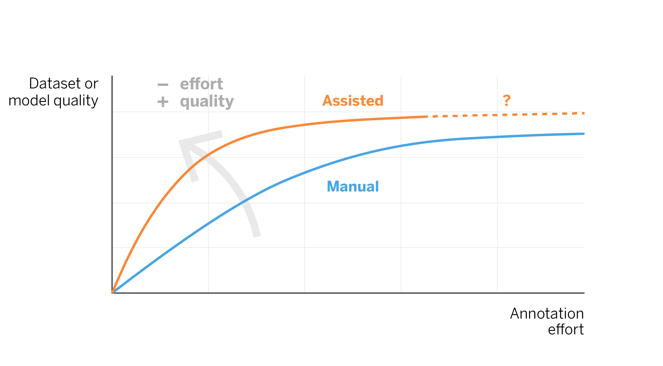
In real autonomous learning applications, the goal is to discover where the boundary is between categories, as we have seen in the previous example. By applying active learning we can do this effectively because it is constantly checking the points near the boundary and correcting the model. It is easy to see how -if we had simply lifted the “boxes” in the example randomly, or for example from left to right and top to bottom-, it would have taken more movements to discover the boundary between the blue and red regions. Therefore, the use of active learning algorithms can result in time saving when labelling data. This gain can be represented theoretically in the following figure.

From example to reality

Although the above animation is a simplified example, the active learning process can be used in real classification applications, for example classifying a conversation. One difference is that in such applications we do not have two attributes (horizontal and vertical position) but hundreds or thousands. For example, in many classification tasks it is common to use one attribute for each word, which takes as its value the number of times it has appeared in a text.

Another difference is the number of categories; for example, in a task of classifying the intent of a conversation there may be dozens of categories, corresponding to the different actions that the user may want to perform. And another difficulty could be that these categories would be non-separable. This would mean that, unlike the previous example where there was a clear boundary between the blue and red regions, samples from different categories would overlap in the attribute space.

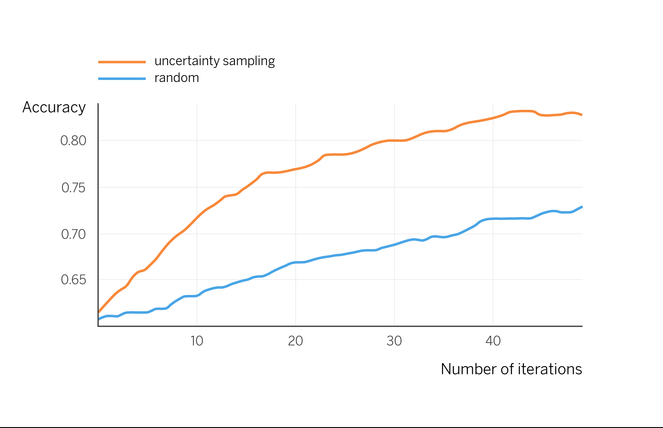
We are going to apply the same active learning mechanism of the example -corresponding to a basic variant called “uncertainty sampling”- to a more complex dataset. We take the public dataset “Banking intents”, which consists of short messages from users requesting to perform one of the 77 possible actions in a banking application. We took 2000 labeled samples to train the first model, and performed active learning iterations for labelling. In each iteration, we ask for 10 new conversations to be labeled, following the uncertainty sampling criterion: those in which the model has more doubts. With the available labels, we simulate how the model would improve as an annotator labels them. We observe how this graph coincides with the theoretical graph shown above, indicating that we would indeed increase productivity in the labelling phase.

Beyond the simple example

The concept of active learning has been proving its viability for decades. Even so, the variant we have explained is the most basic and it is not surprising that in an industrial application it would require more complexity. At the academic level, many other mechanisms have been designed that are more complex than uncertainty samples, for example to adapt them to very recent architectures such as transformers³. There are also certain precautions when deploying these systems industrially and avoiding biases ⁴.

A clear problem of guiding the labelling process exclusively with active learning techniques shown above is that we run the risk of not discovering separation zones between the categories we want to label. Let’s imagine that in the above example of the boxes there is another small set of red boxes in the lower left corner. Our model has discovered that there is a separation of red and blue boxes in the upper right corner, but it focuses too much on that area and we might not discover that in the lower left corner there are also some red boxes. For this reason, it is very important to combine these active learning techniques with a strategy that provides randomness and allows “discovering” behaviors that are not expected by the model, as we can see in the following animation.

In this case, the model is able to detect that second area of red boxes that had initially gone unnoticed. In future articles we will talk in more detail about these more advanced techniques, which improve the final performance of the model.