
AI in finance: budget allocation with Deep Reinforcement Learning
In the dynamic financial landscape, budget allocation remains a significant challenge for portfolio managers. Traditional methods such as fixed-weighting portfolios or Markowitz optimization provide reliable and systematic approaches; however, their rigid characteristics often hinder flexibility in unpredictable markets.
Recent advancements in artificial intelligence have created new opportunities to tackle this challenge, especially through Deep Reinforcement Learning (DRL). This method allows models to learn and adapt by engaging with dynamic environments, making it well-suited for real-time financial decision optimization.
This paper explores the use of DRL on a simplified portfolio of financial assets. Although the results are promising in a controlled environment, this is an academic experiment with which we aim to encourage critical reflection on the potential and limitations of using deep learning in finance.
Budget allocation in portfolio management
Budget allocation in portfolio management refers to the process of allocating financial resources among different assets or investment strategies to achieve financial objectives while managing risk. It is key to portfolio optimization, as it ensures that capital is allocated efficiently based on factors such as expected return, risk tolerance, time horizon and market conditions.
Many funds and financial institutions use fixed-weight budget allocation strategies, but with some variations depending on their investment objectives. Fixed-weight allocation means allocating a constant proportion of capital to different assets or investments, rebalancing periodically to maintain those weightings. These strategies offer significant advantages. On the one hand, their predictability and simplicity facilitate long-term planning, while their consistent allocation to various assets helps maintain stable risk exposure. In addition, they are often cost-effective, thanks to the low fees of passive funds with fixed weightings compared to actively managed funds.
However, fixed-weighting strategies face challenges due to their rigidity, which limits their ability to adapt to market changes. This can cause them to ignore emerging trends or growth opportunities, performing worse in dynamic environments versus adaptive approaches such as those driven by AI or factor-based models.
Optimizing with Deep Reinforcement Learning
In AI Factory we have explored advanced deep reinforcement learning (DRL) techniques to obtain a budget allocation proposal through different financial values (stocks). This optimization problem has several approaches, starting with the development of revolutionary works such as “Portfolio Selection” by Markowitz (1952), which won him the Nobel Prize. Since then, several alternatives have been explored to attack this financial optimization problem.
Inspired by the methodology described in [2] [5], we model the stock market as a dynamic environment, ideal for adapting to rapidly changing conditions. By leveraging historical data, our method identifies strategies that effectively balance risk and reward, offering a robust framework for portfolio management.
This application highlights the transformative potential of reinforcement learning in investment decision-making and financial strategy development, driving innovation in the banking sector. Nevertheless, the content presented in this article is for an informational and research-oriented perspective. This article does not constitute financial advice, investment recommendations, or portfolio management guidance.
In the following chapters we will give a theoretical introduction to the methodology used and then show the results of some simulations made with real public data.
Methodology for Deep reinforcement learning
Advancements in budget allocation within portfolio management have been significantly influenced by the integration of artificial intelligence (AI) and machine learning techniques. A notable development is the application of Deep Reinforcement Learning that combines the strengths of reinforcement learning and deep learning, particularly well-suited for solving complex decision-making problems where an agent learns to achieve goals through trial and error, guided by feedback in the form of rewards.
It is well known that today’s DeepRL algorithms are able to learn advanced strategies, achieved through algorithms such as Deep Q-learning, Policy Gradient, Actor-Critic models, together with exploration/exploitation trade-off. These strategies can also be transferred to industrial applications such as robotics, gaming, finance, healthcare, among others.
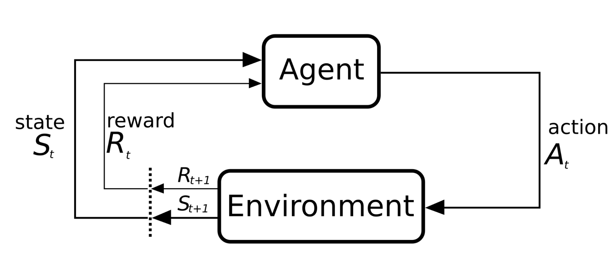
We model the problem as a Markov Decision Process (MDP), a mathematical framework used to model sequential decision-making in uncertain environments, where the outcome of each action is partially random and partially controllable. In this process, the agent observes a state, takes an action, and receives a reward at each time step. This cycle can be visualized as an iterative process in which the agent perceives the environment, acts, and receives feedback to improve its strategy, as illustrated in Figure 1.
- State (St): represents the information available at time t about the market and the portfolio. It includes data such as recent asset volatility (e.g., over 7 and 30 days) and price trends over different time horizons (3, 7, and 15 days). It also considers how the budget is currently distributed among the assets.
- Action (At): is the decision the agent makes on how to allocate the budget across the different assets. This is expressed as percentages assigned to each investment.
- Reward (Rt): is a numerical measure that reflects the outcome of the action taken. In our case, we use a financial indicator that considers the portfolio’s risk-adjusted return, known as the Sharpe ratio.
The agent’s goal is to learn a policy, that is, a strategy that tells it what action to take given a state, in order to maximize cumulative rewards over time. To achieve this, the agent evaluates the consequences of its decisions over multiple steps, balancing exploration of new options with exploitation of strategies that have proven effective.
Furthermore, to prevent the agent from making abrupt changes in budget allocation, a penalty is included to encourage gradual and stable adjustments.
Readers should be aware that the state representations used in the Markov Decision Process (MDP) may be limited and could be enhanced with additional market information or features deemed relevant, and allows the model to detect market shifts. Furthermore, the neural network model can be improved by modifying its architecture to enhance performance and capture more signals from the input states, as long as you carefully monitor performance metrics like overfitting and sensitivity to hyperparameters.
Our experiment with five financial assets
To evaluate the performance of the algorithm, we decided to use five assets, obtaining their historical data using the Yahoo Finance Python library, yfinance: Amazon (AMZN), Alibaba (BABA), BBVA (BBVA), Nvidia (NVDA), and a low-risk asset such as US government bonds.
The selection of these assets is based on their strategic relevance, geographic and sectoral diversification. Including BBVA allows for an analysis of the financial sector’s performance relative to other industries, while US government bonds serve as a low-risk benchmark. These assets reflect key market trends, varying risk levels, and volatility, making them ideal for evaluating and optimizing the algorithm’s performance.
To focus on the core performance of the algorithm, we simplified market conditions by excluding transaction costs in this initial phase. This approach allows us to evaluate the model’s fundamental capabilities before incorporating real-world complexities such as transaction fees. We also decided to compare the effectiveness of the algorithms versus other strategies, such as Equally Weighted Portfolio, and Markovitz portfolio optimization algorithm, where we are maximizing the Sharpe ratio using EfficientFrontier.
The dataset used covers historical data divided into two distinct periods: the training data spans from January 1, 2022, to August 31, 2024, while the testing data covers the period from September 1, 2024, to March 31, 2025. All source code and notebooks required to replicate this exercise are publicly available in this GitHub repository.
Results: smarter allocation
After comparing each of the strategies, starting with a budget equivalent to a capital unit of any currency, after 212 days of test evaluation, our RL agent achieved a remarkable 40.0% profitability, significantly outperforming traditional strategies such as the Equally Weighted Portfolio (22%) and Markowitz Portfolio Optimization (20.0%).
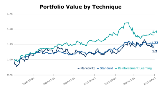
On the other hand, observing the metrics on the following table, the DRL model demonstrates significantly higher average daily returns (0.16%) compared to Markowitz (0.11%) and Equally Weighted (0.10%), with a higher Sharpe ratio and lower Value at Risk at the 95% confidence level. Augmented Dickey-Fuller tests confirm all strategies have stationary returns, validating parametric risk analysis, and supporting the robustness of its profitability.
| Metric | DeepRL | Markowitz | Equally Weighted |
|---|---|---|---|
| Daily Mean Return | 0.16% | 0.11% | 0.10% |
| Annualized Sharpe Ratio | 2.2462 | 1.0464 | 1.5868 |
| Augmented Dickey-Fuller p-value | < 0.05 | < 0.05 | < 0.05 |
| VaR (95%) | -1.38% | -2.39% | -1.65% |
To put this into perspective, the S&P 500 declined by approximately 0.65% over the test period, while the NASDAQ 100 dropped by around 1.51% [6] [7]. While these results are promising, it is important to note that the market conditions in this experiment were simplified, which may affect real-world performance. Nevertheless, the RL model’s performance in this controlled environment appears promising and may indicate potential for real-world applications.
In the below figure, we can see the budget distribution that our agent is making day by day. On the other hand, we can see how the changes in the budget distribution of our RL agent are as little drastic as possible, due to the penalty included in our policy.
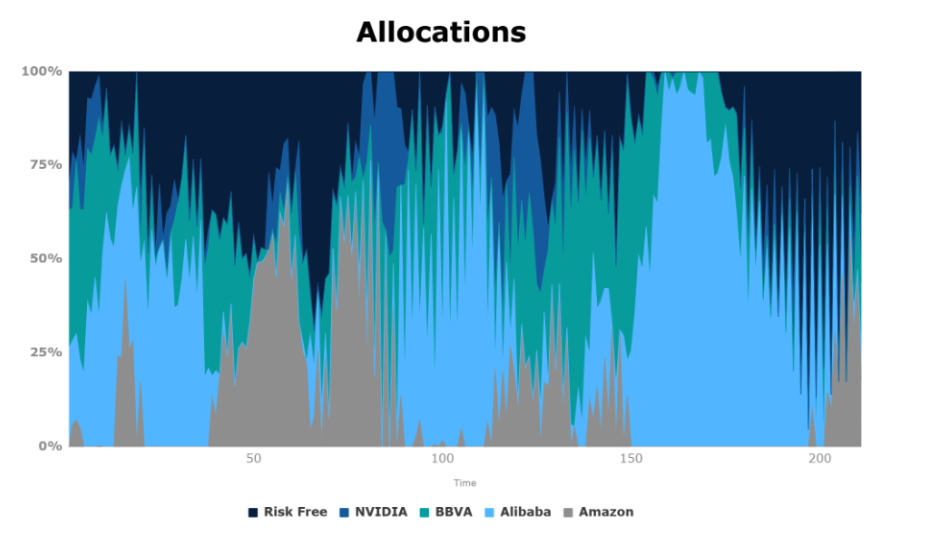
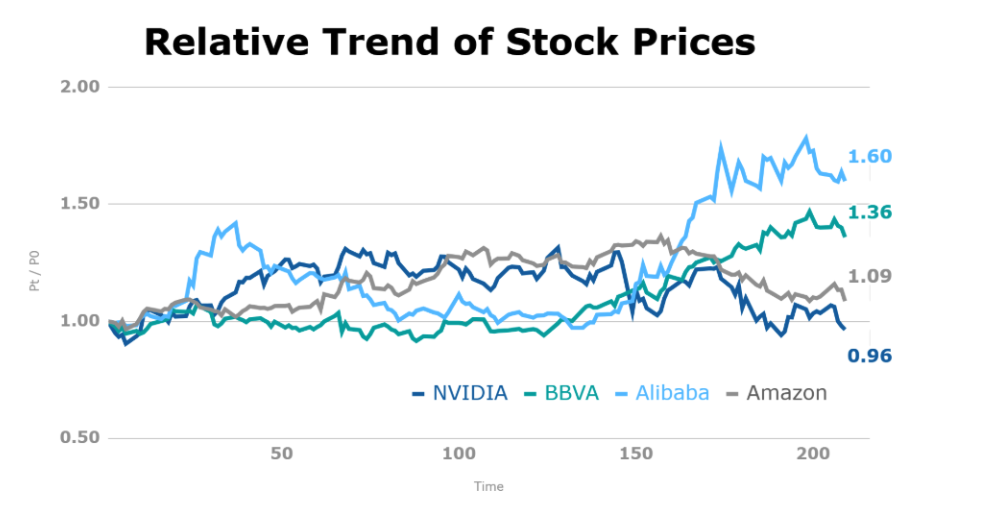
Let’s carefully analyze the decisions made by our agent. We observe that in the case of Alibaba, whose price begins to fall after 40 days (see the below figure), our agent detects it and quickly makes a readjustment in how he distributes the budget, reducing it to Alibaba.
The approach shown is quite simple, in terms of the number of stocks, the signals considered in our state variables, and the assumption of zero fees per transaction. However, we show a way to start using this type of techniques by explaining some theoretical aspects, when using techniques such as DeepRL, for making dynamic decisions in budget distribution.
References
- Richard S. Sutton and Andrew G. Barto, Reinforcement Learning An Introduction, The MIT Press. 2014.
- Yves J. Hilpisch, Reinforcement Learning for Finance, O’Reilly Media, Inc. October 2024. Link ↩︎
- Trade That Swing. Average Historical Stock Market Returns for S&P 500: 5-Year up to 150-Year Averages. Accessed January 14, 2025. Link
- Trade That Swing. Historical Average Returns for NASDAQ 100 Index (QQQ). Accessed January 14, 2025. Link
- Benhamou, E., Saltiel, D., Ungari, S., & Mukhopadhyay, A. (2020). Bridging the gap between Markowitz planning and deep reinforcement learning. arXiv preprint arXiv:2010.09108. Link ↩︎
- AMSFlow. NASDAQ 100 Historical Returns. Accessed April 8, 2025. Link ↩︎
- AMSFlow. S&P 500 Historical Returns. Accessed April 8, 2025. Link ↩︎