BBVA AI Factory | Conformal Prediction: An introduction to measuring uncertainty

Using techniques such as conformal prediction helps us assign confidence levels to algorithmic decisions and, from there, measure uncertainty. Instead of asking, "What will happen?" we start thinking, "What is likely to happen, and how confident are we about it?"

Herodotus and Cicero’s literature has allowed us to preserve the story of Croesus, the king of Lydia. Consulting an oracle, Croesus received a prediction marked by tragic ambiguity: “If you cross the river Halys, you will destroy a great empire.” Convinced that such an omen presaged the fall of the Persian empire, Croesus only realized the double-edged interpretation when it was too late. He crossed the river, and his own empire finally collapsed.

This anecdote drives a lesson that remains relevant despite time: predictions always carry a certain degree of uncertainty, which also applies to artificial intelligence and machine learning.

Placing our trust in these systems should not be an act of faith. Confidence should be based on model robustness and a deep understanding that, while uncertainty will always exist, it can be quantified.

The only certainty is uncertainty

In machine learning, uncertainty can arise from multiple sources and affect all models. It can result from incomplete data, inaccurate measurements, or the inherent variability of the phenomenon we are trying to model.

Thus, the ability to quantify and communicate uncertainty changes the way we interact with technology, allowing us to understand predictions and their limits better. This, in turn, encourages a more critical and analytical approach to decision-making in an increasingly automated and data-driven world.

Conformal Prediction: What is it, and how does it work?

While uncertainty is inevitable, some techniques help us manage it. One is conformal prediction, which gives us a parameterizable level of certainty about a model’s predictions.¹ To understand what it does, let’s imagine that we create a machine-learning model to make recommendations to our clients based on their financial interests.

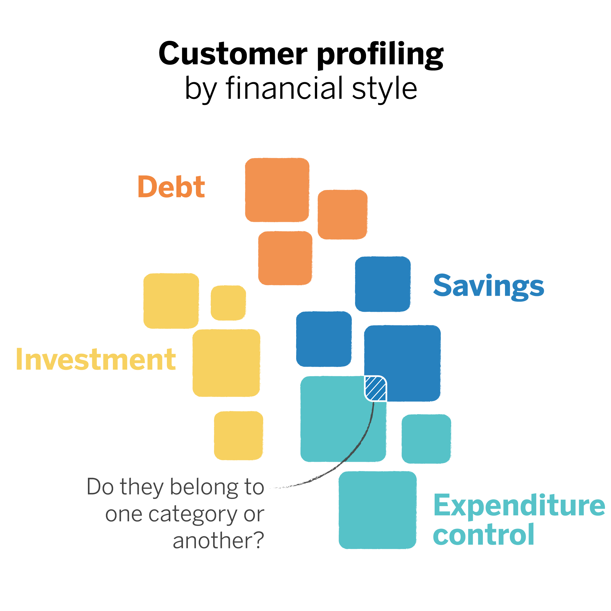
To do so, we start with a classification problem. For recommendations to be personalized, we must classify clients into “investors,” “savers,” and other categories that can help the model associate the financial health recommendation with the right person. However, people can combine several categories, so when classifying them, the model could discern that they belong more to one category than another. In this case, the prediction (“this person is a saver”) would be seen as an unquestionable statement even though it comes from an uncertain fact.

Figure 1. Each square comprises a customer collective. Each collective is associated with a label that identifies customers by what we call their “financial style.” Some customers overlap, so they are associated with one category even though they may belong to both.

In contrast, when we apply conformal prediction, the prediction brings with it a set of possible outcomes, each with its respective confidence levels.²

Suppose a customer has characteristics that may relate to two categories. In that case, the model will tell us they may belong to both and will not categorically associate them with one category. Thus, we would be equipping ourselves with much more knowledge than if we were to stick only with the class with the highest probability.

In this case, a client could fit into a saver or an expenditure control profile. Both categories could be correct, each with a given confidence level. The probability that the client fits the debt profile is substantially lower.

Figure 2. To which category does a customer belong? In this example, on the left, the prediction set comprises {savings, expenditure control} because both classes are “conformal”; both are possible according to the data. The ‘q’ demarcates how far this possibility extends. The class ‘debt’ is excluded on the right because it is too uncertain.

In this sense, the uncertainty lies in choosing one of the two categories for that client, but we avoid associating them with one category and not the other. This could result in the inclusion of new financial recommendations that we may have yet to foresee. The result is a much more reliable classifier, where the prediction’s certainty is guaranteed, and we can clearly see which set of classes is most likely to contain the correct prediction.

Predictive ranges represent a paradigm shift in how we interact with models and interpret them. Instead of asking, “What will happen?” we begin to think, “What is likely to happen, and how sure are we of it?” This shift is crucial in fields where the cost of being wrong is high.

Key concepts

Within conformal prediction, the uncertainty will reside in the fact that different classes may appear within a prediction interval. Unlike point predictions, this knowledge allows us to be discerning. Conformal prediction can be applied in a wide variety of cases, from classification problems to regressions and forecasting.³ We will explore its basic principles to gain a broader understanding of how it works.

Calibration data

They are a specific set of data extracted from the training data and used to estimate the confidence levels of the predictions. The calibration data must be representative of the general distribution of the data to ensure the accuracy and reliability of the predictions provided by a conformal prediction model. The more examples of different casuistries of our problem we add in the calibration phase, the larger the uncertainty coverage spectrum will be.

Non-conformity measures

The basis of conformal prediction is the non-conformity measures. These help us assess how “unusual” a new prediction is compared to the predictions made from the calibration data; that is, they allow us to determine the distance between the new predictions and the set of previous observations, which were used as a reference. Thus, the basic principle is that the more an instance deviates from the previous data, the less “conformal” it will be and, therefore, the higher its non-conformity score will be.

Prediction intervals

This approach uses the previously calculated errors (differences between predicted and actual values) to build confidence intervals around the predictions from the nonconformity evaluation. For a new prediction, the model provides a range or interval within which the actual value is expected to fall instead of giving a single value as the outcome. This interval considers the variability and errors observed previously, trying to capture the true value with a certain probability.

Probability of coverage

The percentage of times that the prediction interval contains the actual value. A coverage probability of 95% means that, on average, 95 out of 100 prediction intervals will contain the true result. Roughly speaking, this value determines the confidence that our model’s prediction contains the correct answer.

Four virtues, the challenge, and a warning

There are other techniques for making predictions with a certain degree of confidence. However, today, we want to highlight the virtues of conformal prediction, keeping sight of what must be considered when applying it, and the challenge it entails.

✨ First virtue: Unprecedented flexibility

One of the main advantages of this technique is its distribution-free nature. Unlike Bayesian approaches and other statistical methods that require specific assumptions about the data distribution (e.g., that the data follow a normal distribution), conformal prediction makes no such assumptions. This flexibility makes it applicable to a broader spectrum of problems, from those with well-understood data distributions to situations with highly irregular or unusual data.

✨ Second virtue: Plug and play

Conformal prediction can be applied to any model; it is model agnostic. From linear regression to deep neural networks, this technique can be used interchangeably, allowing data scientists to use their preferred models or those most appropriate for the task at hand.

✨ Third virtue: Confidence in predictions

This technique’s most distinctive feature is its ability to provide coverage guarantees. For a given prediction region, we can specify with a degree of confidence (e.g., 95%) that the region will contain the true outcome. This probabilistic certainty gives us a tangible way to assess and communicate confidence in our predictions, facilitating informed decision-making and future scenario planning.

✨ Fourth virtue: Adaptability

This technique dynamically adjusts the size of its prediction set depending on the complexity of the analyzed example. Conformal prediction offers smaller sets in situations where the data present clear patterns and are relatively easy to predict. Conversely, the prediction sets are expanded for complicated examples with significantly higher uncertainty.

⛰️ The challenge: Calibration data

In conformal prediction, accurate calibration is essential to ensure that the prediction intervals have adequate coverage properties. The model must be able to adjust its predictions to capture the true distribution of the data, adequately reflecting the level of uncertainty associated with each prediction.

However, different datasets and situations require different levels of adjustment and calibration approaches. A model may work well and be correctly calibrated on one data set but may require significant adjustments to maintain its accuracy on another. This implies that we must have a deep understanding of the data’s nature and the ability to apply calibration techniques that can dynamically adapt to variations in the data.

Addressing this challenge requires a continuous and rigorous evaluation of model performance. Good calibration is a technical challenge and a transparency tool for providing reliable and quality predictions.

⚠️ Warning: Interchangeability assumption

This assumption holds that the data used for model calibration can be interchanged without affecting the probabilities. In many cases, this assumption applies, but in situations where the data have a temporal or spatial structure that breaks the interchangeability, it is necessary to adapt or complement conformal prediction with other approaches to maintain the reliability of the predictions.

How is conformal prediction implemented?

Although there are different algorithms that improve the original idea of conformal prediction, the general method is common to all of them, at least for the most part. The following section will see how it works for a general classification case. Remember, these models tell us the probability that the data we wish to classify (an image, a vector, or another type of input) belongs to each of the available categories. In other words, these models estimate the extent to which an input fits into each category.

Step 0

Before training our model, we must separate a subset of data for calibration, which we will not use during training and validation. Typically, we split the input data in an 80% | 20% ratio, so in this new conformal prediction scenario, we can split it in a ratio of, for example, 80% | 10% | 10%.

Step 1

Next, we train and validate the model using the training and test data. We then review the calibration data and obtain our model’s prediction for each element (class). We keep the probability associated with the actual answer and the category or class it represents among all the probabilities obtained for each prediction.

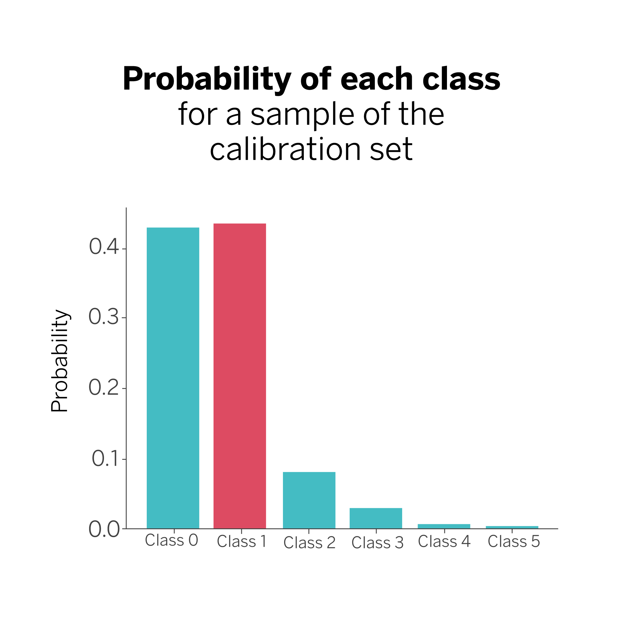
In our example, we have six possible categories to classify each sample. The model then tells us that the true answer in this case is class #1, which typically corresponds to the highest probability, although not necessarily. We may find cases where the probability associated with the true answer is not the highest, but this does not matter. In any case, we will keep the true class and the associated probability ({class 1: 0.44}) for all the examples in the calibration set.

Step 2

We calculate the 0.1 percentile (10%) of all the probability values obtained in the previous step. In our case, that value is 0.42, and we will call it q.

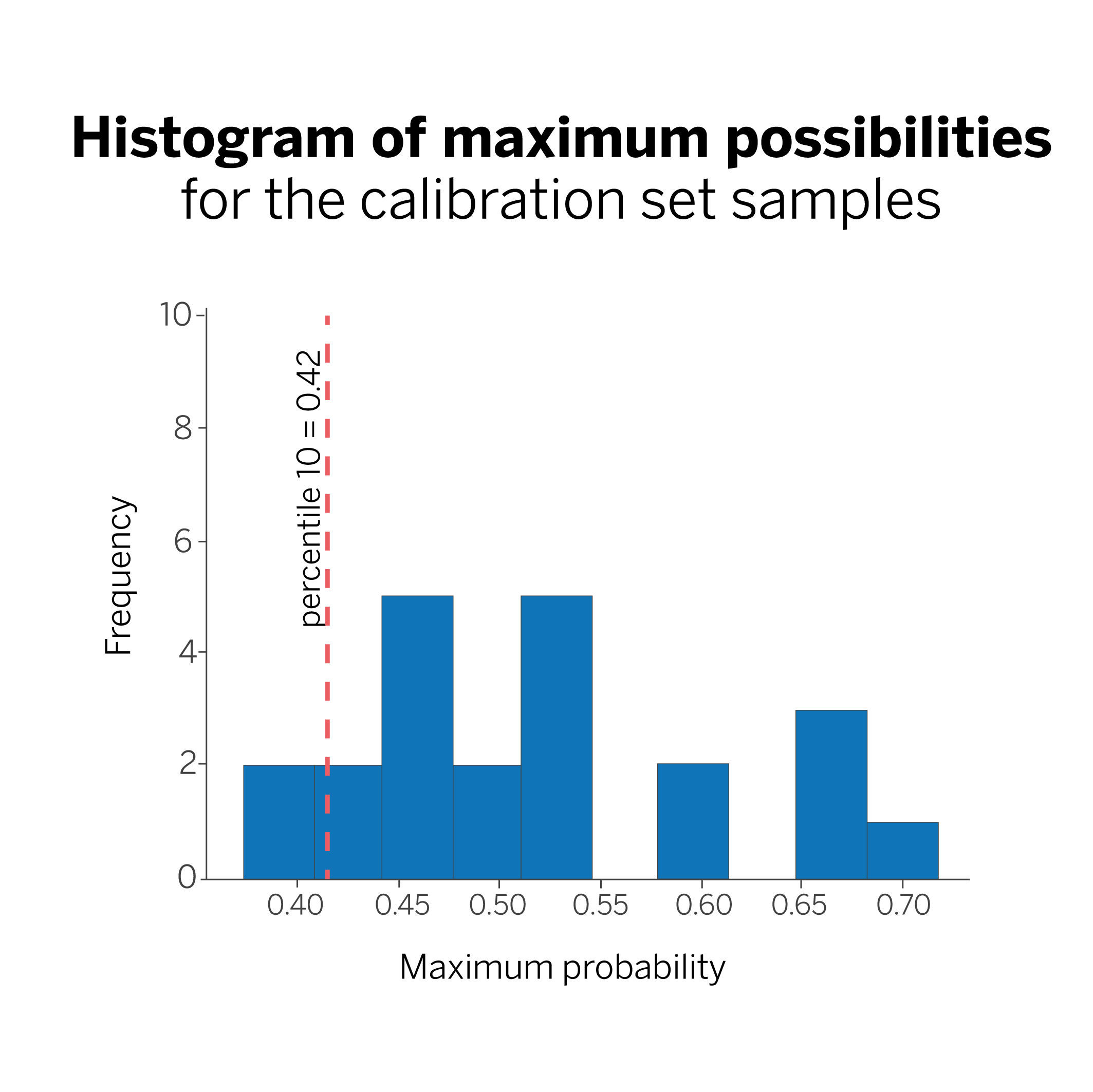
In this figure, the line marking the 10th percentile tells us that we are 90% sure that our model will classify a new sample with a probability greater than 0.42. Why 90%? Because we have chosen the 10th percentile. If we had chosen to calculate the 5th percentile, our coverage would be 95%.

Step 3

We are now ready to make predictions using conformal prediction. When we classify a new sample, all we have to do is ask our model for the probabilities assigned to each possible class to which it may belong and select only those with a value greater than the value calculated for “q.“

In the example, we can see that the probabilities for classes “0” and “1” are above the threshold “q”. In this case, instead of giving class “1” as a prediction, we will say that the sample belongs to the set {“class 0”, “class 1”}; that is, to one of these two classes, with a probability of 90%.

Yes, uncertainty, but make it rigorous

A rigorous knowledge of uncertainty is a way to become strong when faced with predictions’ uncertain nature. This knowledge gives us the information we need to make informed decisions.

Today, Croesus’ dilemma can be interpreted as a metaphor for the ambiguity of predictions made in the form of outright statements: They need to be nuanced, and the real possibilities need to be cautiously weighed. With tools such as conformal prediction, which is finely sensitive to the dynamic nature of data, we can be confident that our day-to-day decisions are indeed the most accurate.

Conformal Prediction: An introduction to measuring uncertainty