
Mercury-Monitoring: analytical components for monitoring ML models
The growth of Artificial Intelligence in recent years has been remarkable. Its sudden proliferation reflects the exponential development of systems based on this technology, which increasingly impacts all spheres of our daily lives. Specifically, at BBVA, we use machine learning solutions to serve our customers daily. These methods allow for the creation of systems such as the classification of banking transactions or the detection of the urgency level of a customer’s message.
Developing these systems involves multiple validations before deploying them to ensure the models function correctly in production environments. However, once a model is implemented, the responsible teams must ensure its proper operation, as these systems often operate in highly dynamic environments. Customer behavior constantly changes, and various circumstances can affect economic activity. Fraudsters also develop new techniques to evade fraud detection systems, among other contingencies.
As a result, the performance of the models can degrade. In other words, the outputs of these systems, which are the results produced by the models, can quickly become incorrect. This increases the risk of causing damage to the business or leading to reputational controversy for the organization.
Model monitoring is an essential practice in the operational phase of a data science project. It helps to detect real-time problems, prevent accuracy degradation in predictions, and ensure that models behave as expected over time. Innovative tools that facilitate such monitoring become essential to guarantee systems’ quality and stability.
Mercury-Monitoring to detect drift and estimate the model’s performance
At BBVA, we have developed Mercury, a Python library that we recently realesed to the entire community. It contains components that have the potential to be reused in various stages of data science projects. The open-source version of Mercury is currently divided into six packages; each focused on a specific topic, which can be used independently.
Today, we dedicate this space to learning more about mercury-monitoring, a package of analytical components specially designed to facilitate monitoring machine-learning models.

This package has been used internally to evaluate the impact of data drift —changes in data distributions— on BBVA’s account and card movement categorizer. For example, during the most decisive stage of the Covid-19 pandemic in 2020, we observed significant deviations in spending categories such as travel, transportation, hotels, and tolls.
In addition, it has helped us monitor drift in generating transactional variables that are later consumed in credit risk models, among many other applications.
We believe that releasing this package as open-source will benefit the entire community and allow for the improvement and extension of its functionalities. Currently, its main capabilities relate to various techniques for detecting data drift and estimating model performance in production when labels are not yet available.
A. Data drift detection
The term “data drift” refers to a situation in which the data received by a model during inference differs from the data used to train the model. This can cause the model to stop performing correctly, leading to inaccurate predictions.
Why does data drift occur?
Data drift can be caused by several factors, including:
- Changes in the environment where the model operates. For instance, deviations in economic activity, new products introduced by competitors, or new fraud techniques created by fraudsters.
- Alterations in some processes, such as variations in the units that provide the model with inputs.
- Changes in seasonality. For instance, if we use a text classifier to identify the subject of customer messages, we may notice an occasional increase in inquiries related to tax returns during the months when they must be filed.
Types of data drift
In most cases, drift detection is performed between two datasets: the “source” dataset, which is typically used to train a model, and the “target” dataset, which is the data that the model encounters once deployed in production.
While many resources describe the different types of data drift in more detail123, in general, we can distinguish between them as follows:
| Concept Shift (or Concept Drift) Occurs when the context for which the model has been trained changes over time. |
Covariate Shift (or Feature Drift) Occurs when the distribution of the input variables of a model changes over time concerning the data used during training. |
Label Shift (or Prior Probability Shift) Occurs when the distribution of the input variables remains the same, but the target variable changes. |
| Example If a model is trained to detect fraudulent transactions, it is deployed in production, and the fraudsters subsequently change their techniques, it will be much more difficult for the model to detect them. |
Example We can consider a model that predicts a customer’s probability of buying a specific product. Suppose customer revenues change once the model has been deployed in production. In that case, the model may become more inaccurate, as it would encounter a different input data distribution than the one it was trained on. |
Example Between 2022 and 2023, interest rates have historically increased due to high inflation. As a result, more and more clients with savings prefer to amortize their loans at variable interest rates partially. Suppose we have a classifier that infers the transaction the client wishes to perform when communicating with his financial advisor. In the current context, it is much more likely that, given the same message content, this classifier will give more probability to the early partial amortization transaction than it would have done before (before the rise in rates, it was an almost residual transaction). |
|
In mathematical terms  even though  The relationship between the input variables of model X and the variable to be predicted Y, changes. |
In mathematical terms  although  Although the relationship between the input variable X and the target variable Y remains the same, the distribution of some input variable(s) changes. |
In mathematical terms  although  Although the relationship between the input variables X and the target variable Y remains the same, the output distribution Y does change (unlike the covariate shift where the input changed). |
1. Concept Shift (or Concept Drift)
Occurs when the context for which the model has been trained changes over time.
Example
If a model is trained to detect fraudulent transactions, it is deployed in production, and the fraudsters subsequently change their techniques, it will be much more difficult for the model to detect them.
In mathematical terms
even though
The relationship between the input variables of model X and the variable to be predicted Y, changes.
2. Covariate Shift (or Feature Drift)
Occurs when the distribution of the input variables of a model changes over time concerning the data used during training.
Example
We can consider a model that predicts a customer’s probability of buying a specific product. Suppose customer revenues change once the model has been deployed in production. In that case, the model may become more inaccurate, as it would encounter a different input data distribution than the one it was trained on.
In mathematical terms
although
Although the relationship between the input variable X and the target variable Y remains the same, the distribution of some input variable(s) changes.
3. Label Shift (or Prior Probability Shift)
Occurs when the distribution of the input variables remains the same, but the target variable changes.
Example
Between 2022 and 2023, interest rates have historically increased due to high inflation. As a result, more and more clients with savings prefer to amortize their loans at variable interest rates partially. Suppose we have a classifier that infers the transaction the client wishes to perform when communicating with his financial advisor. In the current context, it is much more likely that, given the same message content, this classifier will give more probability to the early partial amortization transaction than it would have done before (before the rise in rates, it was an almost residual transaction).
In mathematical terms
although
Although the relationship between the input variables X and the target variable Y remains the same, the output distribution Y does change (unlike the covariate shift where the input changed).
In practice, determining the type of data drift can be difficult. This knowledge is more useful for academia than for industrial applications. Additionally, there may be multiple types of drift coinciding. However, regardless of the type, the most important thing is to detect whether drift exists and take action to mitigate its effects.
What to do when encountering data drift?
The most obvious action when detecting that the performance of our model may be affected by data drift is to retrain it with new data. If we lack mechanisms to detect data drift, we may consider retraining our models regularly with new data. However, in some models, this approach may involve a high computational cost and, thus, not be an effective option.
Other strategies include using adaptive learning models or models that are robust to changes in data distributions.
The existence of data drift does not always imply that model performance is deteriorating, so we also worked on estimating the drift resistance of different machine-learning models.
Which components in mercury-monitoring allow data drift detection?
There are several strategies for detecting data drift in mercury-monitoring. We can distinguish between methods that detect drift by treating each of the variables in a dataset individually and those that consider all the variables together, i.e., their joint distribution.
|
Components to detect drift by observing the variables individually |
Components to detect drift by observing the variables jointly |
These components provide a boolean or binary (yes/no) result of whether drift has been detected or not, as well as a score indicating the amount of drift. This allows monitoring of the data over time. |
|
Components to detect drift by observing the variables individually
- KSDrift: performs a Kolmogorov-Smirnov test for each variable. If it detects drift in at least one of them, the drift detection result will be positive.
- ChiDrift: similarly, this test performs a chi-square test of independence between distributions for each variable.
- HistogramDistanceDrift: In this case, the distance between histograms is calculated for each variable. This is done to detect if there is drift in them. This distance can be calculated in different ways. For example, using the Hellinger Distance or Jeffrey’s Divergence is possible.
These components provide a boolean or binary (yes/no) result of whether drift has been detected or not, as well as a score indicating the amount of drift. This allows monitoring of the data over time.
Components to detect drift by observing the variables jointly
- DomainClassifierDrift: trains a classifier to distinguish between samples that come from the reference dataset (the training dataset) or the inference dataset. If the classifier performs well enough, the component will indicate that drift has been detected.
- AutoEncoderDriftDetector: This method is based on autoencoders. First, several samples are taken from the reference dataset by bootstrapping sampling. Then, an autoencoder is trained on each of these samples, and the reconstruction error distribution is saved for each autoencoder. Subsequently, when the inference dataset is available, the reconstruction error distribution of this dataset is calculated and compared with the distribution obtained in the reference dataset. A Mann-Whitney U-test is used to decide whether drift exists or not.
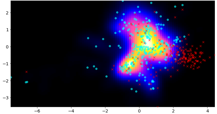
- DensityDriftDetector: This method calculates the probability that a sample is anomalous concerning a reference dataset. It uses Variational AutoEncoders to build embeddings and estimate a density so that areas of the space with many embeddings have a high density. In contrast, areas with a low density of embeddings have a low density. In this way, if an inference sample is embedded in an area with low sample density, it can be considered more likely to be an anomaly.
B. Estimating the performance of a label-free model
Sometimes, after deploying a model in production and it starts making predictions, we are unsure of how well the model will perform on new data. This is because we have no information about the actual labels.
This situation can occur, for example, when offering a product to a customer, since it may take some time from when it is offered to when it is purchased. Another example is when predicting the risk of non-payment of a loan: until it has been paid, it is impossible to know whether the model has made a correct prediction.
How to improve model performance estimation with Mercury-monitoring
Mercury-monitoring offers a component that can predict the performance of a model even when the labels are unknown. This method is based on the paper Learning to Validate the Predictions of Black Box Classifiers on Unseen Data4. Given a trained model, the following steps are followed:
- Corruptions are applied to a test dataset to obtain labels.
- Percentiles of model outputs and model performance are obtained when those corruptions are applied.
- The regressor is trained using the obtained samples to predict the performance of a model.
- The regressor is used to estimate the performance of a model with unlabeled data during inference.
Although this method may not always predict performance accurately, experimental studies have shown that it can detect drops in model performance under various circumstances, thus confirming its usefulness for performance estimation.
Let’s try it!
Mercury-monitoring is available in Pypi and the easiest way to install it is using pip:
pip install -U mercury-monitoring
After installing the library, a good way to get started is to review some tutorials or visit the documentation. Additionally, visting the repository to understand better how the components work internally is advisable.
Conclusions
Monitoring the models we deploy in production is critical to understanding their performance, receiving feedback, and iterating accordingly. Situations such as data drift can impact most machine-learning systems. Therefore, having tools to detect performance drops in our models helps us proactively maintain their correct operation in production environments.