
Smoothing risk: A Machine Learning pipeline for early debt recovery
The core business of the bank is lending money. Through the repayment of installments, financial institutions enable people to buy homes, buy cars, or start their own entrepreneurship. However, when clients face adversities and fall behind on their payments, an unfavorable situation can arise for both the bank and its customers.
At AI Factory, we develop predictive models for early debt recovery in various scenarios. The goal is to assist the client in quickly overcoming or preventing the worsening of this unfavorable situation.Thanks to these models, the bank can offer early solutions, such as refinancements and adjusting installments into affordable fees.
Today, we want to share how we develop models aimed at debt recovery. To do so, we employ state-of-the-art ML techniques in the context of supervised learning with tabular data.
Specifically, we have created a pipeline in which we automate various standard processes throughout the different debt recovery models we develop. It combines traditional risk analysis methods with the latest in supervised learning libraries.
Our Use Cases: Different ML models to address different debt states
Customers can find themselves in various states concerning their debt payments, for which we apply different data models. All these models assist BBVA’s managers in deciding as soon as possible what actions to take.
| Debt status | Up-to-date on payments. | In irregular payment status, when they have some overdue installments for less than three months. | In default, when they have failed to pay one or more installments for three months or more. |
| Models | 1. Model for predicting entry into irregular payment status. | 2. Model for predicting exit from irregular payment status. | 3. Model for predicting exit from default in a short period (45 days). 4. Model for predicting prolonged default (not exiting default within two years). |
| Debt status | Models |
| Up-to-date on payments. | 1. Model for predicting entry into irregular payment status. |
| In irregular payment status, when they have some overdue installments for less than three months. | 2. Model for predicting exit from irregular payment status. |
| In default, when they have failed to pay one or more installments for three months or more. | 3. Model for predicting exit from default in a short period (45 days). 4. Model for predicting prolonged default (not exiting default within two years). |
Why a Machine Learning pipeline for debt management?
Traditional mathematical models, such as logistic regressions, are still applied in the field of risk analysis. These models are simple and very interpretable; however, sometimes, they don’t reach the performance levels other non-linear ML methods can. At AI Factory, we aim to find a balance between the more traditional methodologies standardized in risk, which help us have a reference starting point, and innovative techniques that allow us to create productive models with greater predictive power by contrasting both methodologies.
In addressing various debt recovery problems and applying ML models to solve them, we realized the same steps were continually repeated. We decided to unify these phases into our debt management modeling pipeline to be more agile, allowing us to reuse code and automate processes across different projects.
We start from some premises:
| Our models focus on supervised learning with tabular datasets to predict variables, which are usually binary. | |
| We need to consider a good amount of variables – more than 1800 in some cases – which include behavioral, sociodemographic, transactional, and debt level data. The data’s diversity and volume demand a consistent dimensionality reduction process. | |
| We face tight deadlines and must build and validate effective models beforehand. An automated pipeline significantly accelerates this process. | |
| It’s essential to create explainable models that allow us to interpret their results, thereby translating them into business language. | |
| Score segmentation is necessary for precise evaluation and adaptation to different contexts. |
Our pipeline’s standardization helps us reduce the Time To Value, i.e., the time we take to add value, when we start a new project with the same business area. Also, as we develop new products and reuse this pipeline, we find improvement points and update them.
Our Proposal: Zooming in our Machine Learning Pipeline
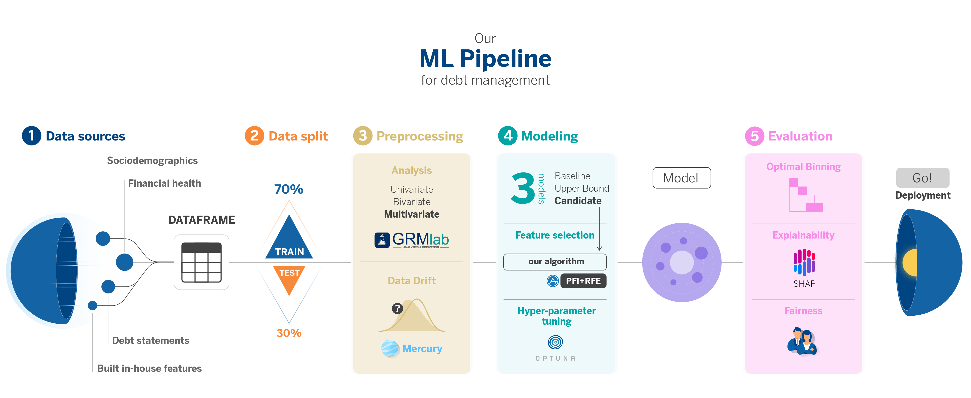
We will go through all the stages of our pipeline, covering the complete lifecycle of building a model. This process begins with the data board generated in the ETL phase and ends with implementing the optimized model, ready for deployment in production environments.
Throughout this journey, we will mainly focus on those phases that present greater technical complexity and in which we have explored new, less-known libraries that facilitate the work or improve the already known ones.
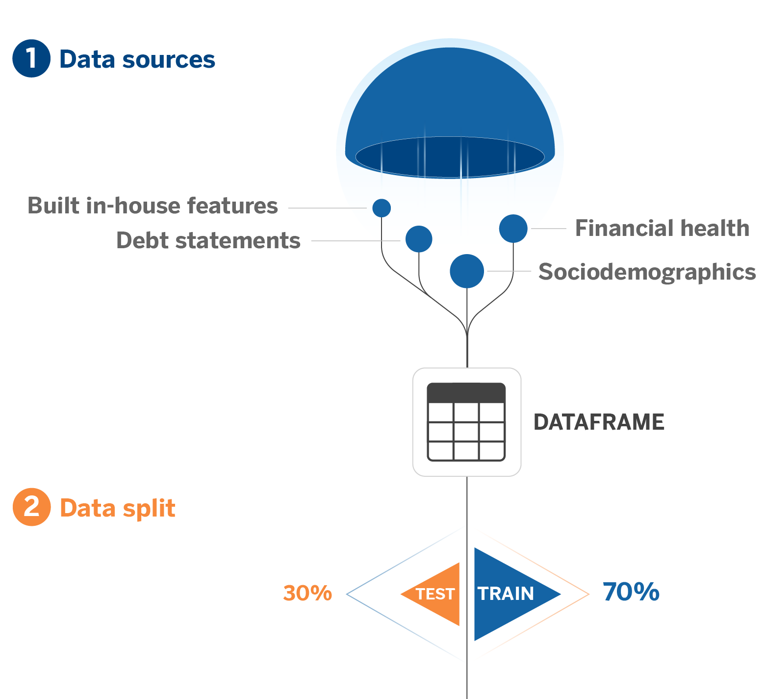
1. Dataset Construction: ETL (Extract, Transform, Load)
The first step is the construction of the data board. As mentioned, most problems we solve involve tabular data, which implies building a table through an ETL using the different available data sources.
We use sociodemographic variables, financial behavior, debt situation, and some other variables generated through feature engineering, depending on our target variable. The final board includes the target and all the variables we want to use to predict it.
2. Data Split
Next, we perform data splitting and variable selection as in any ML project. We make an initial split between data designated for the training, validation, and test phases. The test sample’s data responds to a chronological split. It includes the most recent data, so we have a clear reference of how the model will perform in production by simulating an inference scenario.
3. Preprocessing
Subsequently, we perform univariate, bivariate, and multivariate analyses on variables using GRMLab, an internal tool for the development of models for BBVA’s Risk area. This way, we preselect them, narrow down their number, and, thus, optimize the dataset for modeling.
The next crucial step in our process is identifying data drift, aiming to eliminate variables whose distributions vary significantly over time. This action is essential to prevent the model’s degradation in production environments and reduce the risk of overfitting, ensuring the model generalizes well. In short, the goal is to develop a stable and robust model.
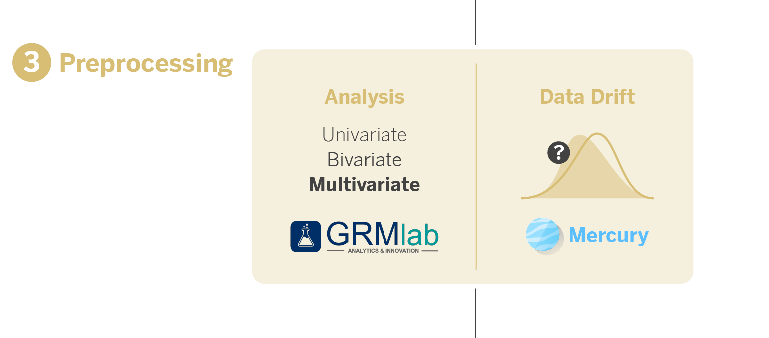
We use advanced algorithms from the open-source library Mercury to tackle this challenge. Mercury, developed by some of our colleagues at AI Factory, is notable for providing innovative and efficient tools to simplify and accelerate ML model creation.
Mercury-monitoring includes two specific algorithms designed for detecting changes in the distribution of variables at both univariate and multivariate levels. This helps us identify and discard variables whose distribution changes significantly before proceeding with model building.
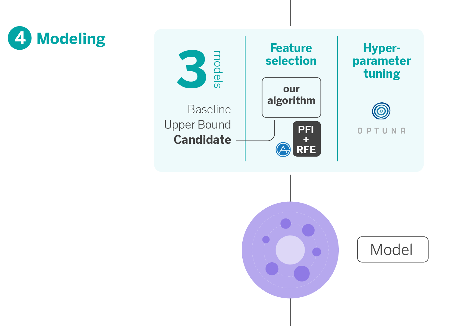
4. Modeling
In this stage, our pipeline generates three models, each with a specific purpose.
- Baseline Model: This model is based on traditional risk methodology and serves as a benchmark for minimum performance. We simulate the approach that would have been applied with conventional techniques like logistic regressions.
- Upper Bound Complex Model: We build this model using AutoGluon1, an open-source AutoML library created by AWS that stands out for its ability to generate models very agilely and make them highly predictive, with few lines of code from “raw” data. This model acts as a performance ceiling, showing us the maximum predictive potential. It comprises an assembly of multiple layers of models to make it highly effective. However, its intricate nature makes it complex for direct implementation in Risk’s strategic infrastructure, mainly due to its lack of transparency and interpretability, critical aspects for communication with business.
- Candidate Model: This is the model that is actually employed. Selecting the candidate model involves finding a balance between the type of algorithm, variable selection, and hyperparameter optimization. Given time constraints and computational resources, we develop a sequential solution that addresses these three aspects efficiently. We start with a list of compatible algorithms with our environment and proceed with time series cross-validation to ensure solid and realistic performance.
Each of these models plays a crucial role in our modeling strategy, ensuring that the final model is robust, interpretable, and suitable for implementation in a real banking environment.
Selection of finalist variables
Feature selection is fundamental, especially when working with large datasets. The objective is to identify and discard redundant variables that do not provide significant information to the model.
We have tons of variables; that’s a fact. As it is computationally impossible to eliminate variables one by one in different iterations and optimize the model’s hyperparameters at each step, we use a technique called PFI+RFE2, developed by AutoGluon, to eliminate redundant variables more efficiently.
Hyperparameter optimization
Optimizing hyperparameters is essential to ensure optimal model performance when deployed in production. Within our modeling process, we have explored various state-of-the-art methodologies and frameworks to improve the efficiency of our models:
- AutoGluon: As previously explained, this AutoML framework developed by Amazon AWS has been trained with many datasets. It starts the hyperparameter search from initial values that generalize very well (transfer learning). Since the starting point is good, searching for optimal hyperparameters is faster. It also offers various search algorithms, including Random Searcher, Bayesian Optimization, and Reinforcement Learning Searcher.
- FLAML: An AutoML library developed by Microsoft, FLAML generates various combinations of hyperparameters within the defined search space. It starts the search with a less complex and quicker training combination, gradually training with increasingly complex and computationally expensive combinations, adjusting to a predetermined time budget, and adding as much complexity as possible. In short, it’s an efficient method that reduces computational costs without affecting convergence towards the optimal solution.
- Optuna: A framework focused on hyperparameter optimization. It allows complete customization of the objective to be optimized and the hyperparameter search space. It also helps select a random or temporal train/test split (time series cross-validation). The process begins by defining a customizable objective function and a search space. Then, we choose a hyperparameter algorithm that iterates the same number of times as the selected trials. One of its major advantages is its capacity for multi-objective optimization.
Given the nature of our use cases, we opt for this last framework for our pipeline. It allows us to maximize the AUC (Area under the ROC Curve) and minimize overfitting3. We also chose it for allowing time series cross-validation, which, for instance, AutoGluon and FLAML do not permit.
With these methodologies, once the optimal algorithm is selected, the Permutation Feature Importance is completed, and the hyperparameter optimization is finished, we obtain a solidly configured candidate model ready for practical implementation. But, before that, it is necessary to evaluate it.
5. Evaluation module
This module is a vital stage in our modeling process, where we thoroughly evaluate the model to ensure it is accurate, understandable, and fair. Hence, it meets the needs and diversity of our clients and aligns with our ethical and business standards.
It’s an exhaustive evaluation module, which allows us to identify any problem the model might have and backtrack in time, if necessary, in any of the previous steps. In this phase:
- We perform a global evaluation of the model. We use metrics like the Gini index4, recall, and confusion matrix to assess the model’s overall performance.
- We segment the metrics. Not all clients are the same, so we also evaluate the model by segments, such as the type of financial product or the client’s refinancing history. This helps us understand how the model performs for different client groups.
- We measure temporal stability and drift. We verify that the model maintains its performance over time and that there are no significant deviations (drift) in the data, which is crucial for its long-term applicability.
- We apply Optimal Binning for risk management. Instead of using a single threshold for risk decisions, we employ Optimal Binning to discretize the model’s score into intervals. This allows the business unit to offer specific actions according to the client’s criticality.
- We interpret through explainability techniques. We use the SHAP library to understand the impact of the variables on the model. This helps us interpret the model’s behavior and effectively communicate its functioning internally and with business stakeholders.
- We evaluate fairness. We conduct a fairness analysis to ensure that the model does not engage in gender discrimination.
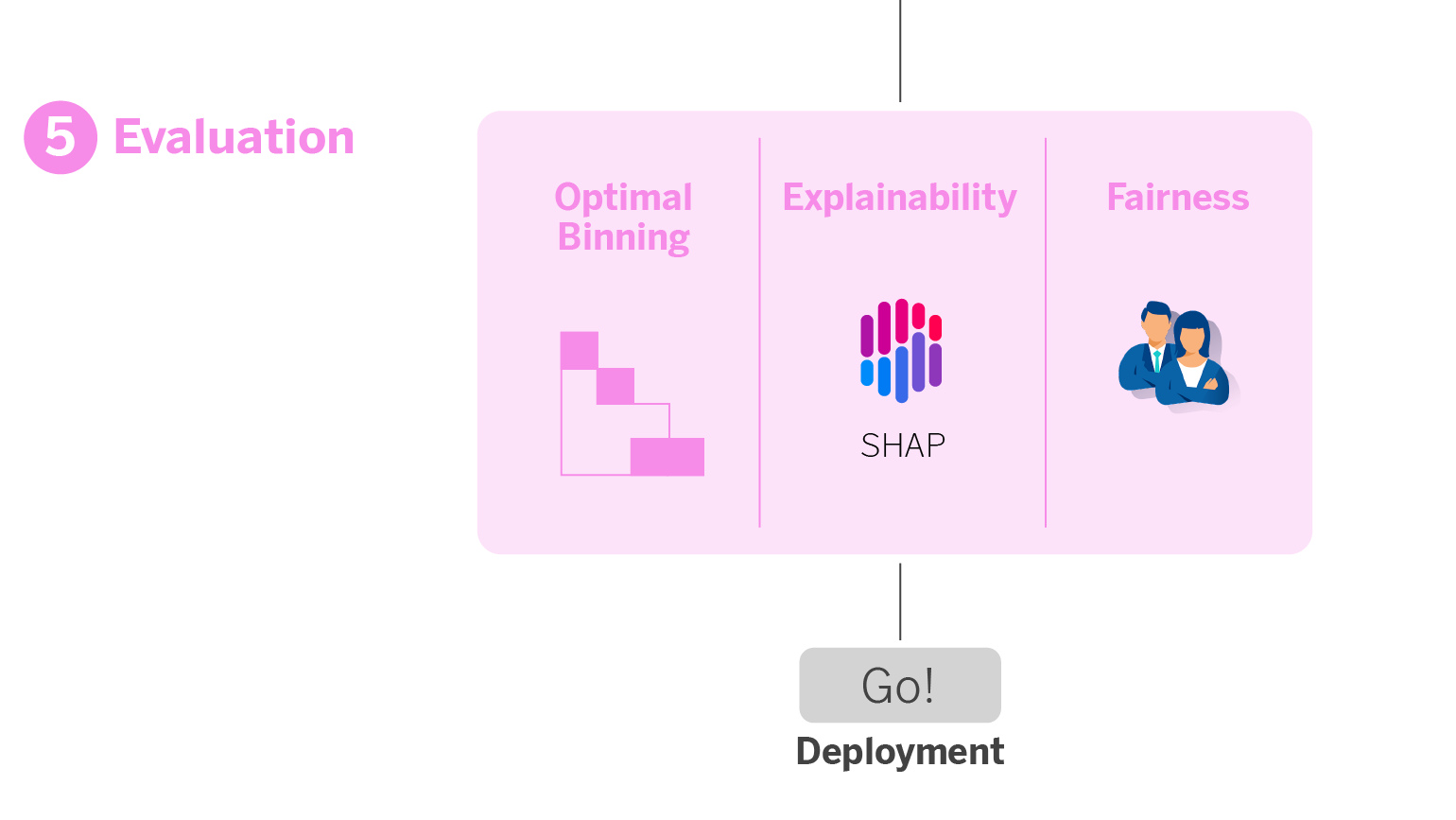
6. Deployment!
If all the analyses designed in the previous evaluation module are correct, we now have the model ready for production deployment. Next, it’s essential to monitor the model’s performance to track it over time and ensure there is no data drift; in this case, it will need to be retrained.
Takeaways: Where does the differential value of our pipeline reside?
At first glance, the phases of our pipeline might seem like any other. What makes the difference is the inclusion of various state-of-the-art libraries –both external and internal (GRMLab and Mercury)– that can help streamline the development process, gaining precision and maximizing predictive power. Below you can find a list of the open-source libraries used in each phase of our pipeline.
Algorithm Selection
AutoGluon, to create models with a high predictive level from raw data with few lines of code in less time. This allows comparing the performance and overfitting of different algorithms to choose a winner.
Selection of Finalist Variables
PFI+RFE, from AutoGluon, to efficiently eliminate redundant variables or those that add little information.
Hyperparameter Optimization
Flaml, to tailor hyperparameter search times to your needs.
AutoGluon, for finding optimal hyperparameters much faster.
Optuna, for customizing the hyperparameter search according to your goal, allowing you to define more than one.
Evaluation Module
SHAP, for a broader understanding of the impact of variables on the model and to better explain it to business professionals.
Monitoring
Mercury-monitoring, to ensure that your models in production maintain their performance over time and alert in case of model deterioration so you can retrain accordingly.
Conclusions: Tradition-innovation symbiosis to create productizable models
The pipeline we dissect here has allowed us to streamline the process of developing debt management models; however, this pipeline can be used in any use case involving supervised learning.
We achieve greater precision and efficiency by applying new state-of-the-art libraries in the traditional ML product development cycle phases – a perfect symbiosis between tradition and innovation.
Notes
- Its modeling methodology consists of training layers of models and assembling them by means of multilayer stackings. It trains several models in the first layer, from which it obtains some predictions that will be the features that go to the next layer and with which the following models will be trained. And so on until the predefined number of layers is reached. At the same time it does bagging, that is, it trains each of the models with a k-fold CV and passes the out-of-fold predictions to the next layer to try to mitigate the overfitting generated by passing the predictions of the training set. To all this, we must add the hyperparameter optimization performed in each model. ↩︎
- This approach starts by permuting the variables one by one, several times, and evaluates how each permutation affects the performance of the model. If the performance does not change significantly after permuting a variable, we conclude that that variable contributes little information. Conversely, if the permutation causes a large loss in performance, it means that the variable is important. The variables are then ranked according to their importance and progressively eliminated in blocks, evaluating at each step the impact on performance. This process is repeated until no more variables can be discarded without negatively impacting the model. In this way, we manage to significantly reduce the number of variables while maintaining the efficiency of the model.↩︎
- Most models with better validation metrics tend to have higher overfitting, in addition to quite complex parameterizations that can lead to robustness problems and performance degradation over time.↩︎
- The Gini index is the benchmark metric used for its ability to measure the model’s ordering power, which helps determine how effectively the model can identify predetermined observations based on the order of its predictions. This allows us to compare the performance of various models.↩︎